Tomographic Inversion Technique Using Orthogonal Basis
Patterns
∗
)
Satoshi OHDACHI
1,2), Satoshi YAMAMOTO
3,a), Yasuhiro SUZUKI
1,2), Shishir PUROHIT
2)and Naofumi IWAMA
1)1)National Institute for Fusion Science, Toki 509-5292, Japan
2)SOKENDAI (The Graduate University for Advanced Studies), Toki 509-5292, Japan
3)Institute of Advanced Energy, Kyoto University, Uji 611-0011, Japan
(Received 17 January 2019/Accepted 18 March 2019)
Tomographic reconstruction of the emission profile is a typical ill-posed inversion problem. It becomes trou-blesome in fusion plasma diagnostics because the possible location/direction of the observation is quite limited. In order to overcome the difficulty, many techniques have been developed. Among them, series expansion meth-ods are based on decomposing the emission profile with orthogonal or nearly orthogonal basis patterns. Since it is possible to ignore the surplus components with higher spatial frequency, this type of method is robust against noise issues. Two topics are discussed in this article. The first issue is the comparison of the basis systems them-selves. Conventional one of Fourier-Bessel and a new one of the so-called Laplacian eigen function are compared from the viewpoint of the capability of expressing the patterns that appear in the fusion plasma experiment. The second issue is the application to the tangential viewing imaging system. It is shown that, even from the limited information, tomographic reconstruction can be adequately performed with appropriate use of the regularization, especially with the use of the L1 regularization.
c
2019 The Japan Society of Plasma Science and Nuclear Fusion Research
Keywords: tomography, Heliotron-J, orthogonal, series expansion DOI: 10.1585/pfr.14.3402087
1. Introduction
Diagnostics using the tomographic reconstruction in fusion plasmas reveals many important physics, such as the mechanism of the MHD instabilities [1]. However, it is not straightforward to reconstruct the local emission profileg from the line-integrated signalsf since it is a kind of ill-posed problem. With column vectorsfandg, thefcan be expressed as
f=Hg+(Noise), (1)
using the geometrical relationship expressed as the matrix H.
If the least square fitting method is used to solve Eq. 1, the following minimization may give the solutiong:
arg min g {
g| i
(fi−hi·g)2}, (2)
wherehiis the i-th row vector of the geometrical matrix H. If this solution is ill-behaved and unstable to the noise, an additional penalty function is often introduced. When the penalty function is concerned with the total magnitude of
author’s e-mail: [email protected]
∗)This article is based on the presentation at the 27th International Toki
Conference (ITC27) & the 13th Asia Pacific Plasma Theory Conference (APPTC2018).
a)Current affiliation: National Institutes for Quantum and Radiological
Science and Technology, Naka 311-0193, Japan
the local emission, the function to be minimized becomes Eq. 3.
arg min g {
g| i
(fi−hi·g)2+λ
i
|gi|α}. (3)
Whenα =2, the penalty function is the squared Euclid norm of the vectorg. This regularization scheme is called the L2 regularization (Ridge regression). Whenα = 1, the scheme is called the L1 regularization (least absolute shrinkage and selection operator (Lasso) regression). Re-cently the algorithm for L1 regularization is significantly improved and widely used for the regression problems in various fields research.
On the other hand, in the large-scale fusion devices such as JT-60U, JET, and LHD, the possible location for the detectors are quite restricted. The coverage of the sight-lines may be therefore insufficient. That is to say, the re-construction with lesser information is required in the large scale experiments and in the next generation devices. That means the tomographic reconstruction method should be improved in the scheme of numerical estimation.
The series expansion method using global orthogonal basis patterns was a method proposed in the early stage of fusion research [2]. This method was quite effective for reconstructing the emission profile, especially, of the Toka-mak plasmas in circular cross section. Since this method is based on the global patterns, it might be possible to
re-c
2019 The Japan Society of Plasma
construct the emission profile from the information that is acquired by the measurements of much limited coverage of the entire objective region. However, the application of the series expansion method to the non-circular cross section devices has not been studied intensively. The capability of the reconstruction using the global basis patterns is inves-tigated in this article.
In the series expansion methods, the emission profile gis expanded by a series of patternsbias
g= i
βibi, (4)
that is, we have a series expansion offwith basis patterns xi=Hbi:
f= i
βixi. (5)
The coefficientsβiare determined from the measure-ment by minimizing the β = arg minβ{i(fi −βixi)2 + λi|βi|α}. With the obtained coefficientsβi, the local emis-sion profilegcan be easily composed using Eq. 4.
This article is organized as follows. First, basis pat-tern calculation that is adaptive to the complicated flux sur-face is introduced. The capability of the calculated patterns to express the complicated emission profile, which are of-ten observed in the fusion experiments, is investigated in Section 2. Second, this method is applied to the specific tomographic reconstruction problem (tangentially viewing camera system), and the performance of the reconstruction is studied in Section 3.
2. Image Composition Using
Fourier-Bessel Series and Laplacian Eigen
Function Series
Two types of basis patterns are examined in the ca-pability of composing an emission profile. The objective geometry is of the Heliotron J device having a non-circular poloidal cross section. The Heliotron J is a medium sized helical axis Heliotron with L/M=1/4 [3,4]. It is noted that the analysis using Phillip-Tikhonov regularization [5] has been already executed [6].
Figure 1 shows the patterns for expansion. The first type of patterns are produced from the Fourier-Bessel se-ries which is used in the solution to partial differential equations, particularly in cylindrical coordinate systems. The series of patterns are expressed as
Ψm
l(ρ, θ)=exp(imθ)Jm(λlmρ). (6) Here, Jm is the m-th Bessel function of the first kind whereλl
mis thel-th zero location of the m-th Bessel func-tion. θandρare the coordinate in poloidal direction and the averaged minor radius, respectively. It is noted that this series satisfies Dirichlet’s boundary conditionΨm
l (ρ= a, θ) = 0 at the boundary of the plasma. In order to pro-duce the series of patterns fit to the Heliotron J equilib-rium shape,ρandθin VMEC coordinate [7] are used for
Fig. 1 Basis patterns for expansion: FB patterns with l = 0 (Figs. 1 (1a) - (1e)) andl=1 (Figs. 1 (2a) - (2e)) and LE patterns for the four largest eigen values (Figs. 1 (3a) -(3d)) and the 30th eigen value (Fig. 1 (3e)).
Eq. 6. The orthogonarity of the Fourier-Bessel functions is not completely maintained through this mapping. The Fourier-Bessel series withl =0 (Figs. 1 (1a) - (1e)) andl
=1 (Figs. 1 (2a) - (2e)) are shown in the sequence of the poloidal mode number.
Another candidate for the basis pattern is the so-called Laplacian eigen function (LE) [8]. The fundamental solu-tion of the Laplacian in two dimension is,
k(r1,r2)=− 1
2πlog|r1−r2|. (7)
The integral operatork has the following eigen function expansion [9],
k(r1,r2)∼
∞
j=1
μjφj(r1)φj(r2). (8)
This series of eigen function is easily calculated when equation 7 is discretized to the matrix form. The advan-tage of this expansion is that a series of orthogonal pat-terns can be produced for any shape of the objective region. Thus, this method of pattern production is widely used in the pattern recognition study and the visualization of the fluid dynamics. Figs. 1 (3a) - (3e) show the orthogonal pat-terns made by this Laplacian eigen function scheme.
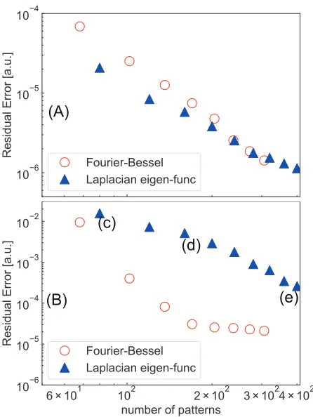
from 2 to 20. For Laplacian eigen function, 400 patterns having the largest eigen values are used. Residual error for peaked profile (Fig. 3 (A)) and the magnetic island-like profile (Fig. 3 (B)) are shown as the function of the number of patterns used for decomposition.
Both basis patterns give adequate decomposition though the patterns of the LE are rather unfamiliar types of shapes. In the case of the island type patterns (Fig. 2 (b)), reduction of the residual error is quicker for FB type patterns. However, composition with LE behaves well when a sufficiently large number of the patterns are used. Even when the insufficient number of patterns are used (e.g., Fig. 2 (c)), the composed pattern represents the ba-sic feature of the island-like emission pattern. Better performance of the FB type patterns is caused by the
Fig. 2 Patterns to be composed are shown in (a) and (b). The emission profile is exp(−(ρ/0.5)2) ×(1−ρ10) (a) and
exp(−((ρ−0.8)/0.1)2)∗cos(2θ+0.2π) (b). The change of
the composed profile with LE shown in (c), (d) and (e). Number of the patterns used are plotted in Fig. 3 (B).
Fig. 3 Change of the residual error in composing (A) the peaked emission profile and (B) the island like emission profile.
fact that the island like structure are constructed on the equilibrium flux surfaces. A small number of num-bers of patterns are therefore required for reconstruction (Fig. 3 (B)). In these decomposition, the coefficientsβi es-timated with L2-type regularization.. The renormalization parameterλwas determined by minimizing Akaike’s in-formation criterion(AIC) which was evaluated asAIC = nlog(residual error)+2d f. Here, n is the size ofgand the freedomd f was evaluated byd f =λiλi+λ whereλiis the eigen values of thexTxforxin Eq. 5 [10].
It is concluded that both basis patterns are appropriate for the composition of the emission profiles routinely ob-served in the fusion experiments. If we know the shape of the flux-surfaces beforehand, the performance of the FB type may be better. However, the merit of the LE where only the boundary shape is required to construct basis patterns, is also quite attractive in the fusion experi-ments when the detailed equilibrium shape cannot be deter-mined in advance. Although the LE patterns do not satisfy Dirichlet’s boundary condition, it is found that the compo-sition of the profiles having zero emission at the boundary can be free from significant error.
3. Application to the Tangential
View-ing System
As an application of the series expansion method, re-construction of the local emission profile from the tangen-tially viewing camera image [11] is discussed in this sec-tion. Figure 4 shows the arrangement of the virtual di-agnostics, where a diagnostics system having two tangen-tially viewing camera observing a torus plasma having a circular cross section. This arrangement is similar to the situation where two tangentially viewing SX camera
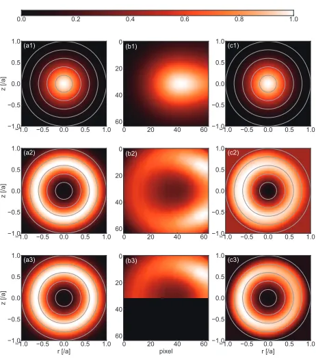
Fig. 5 The emission profile assumed is shown in Figs. (a1), (a2) and (a3). Emission profile of exp(−(ρ/0.3)2) is assumed
in (a1) and exp(−((ρ−0.7)/0.05)2) in (a2) and (a3).
Syn-thetic images from (a1) - (a3) are shown in (b1) - (b3). Reconstructed images are shown in (c1) - (c3). For (c3) only upper half of the tangential image of (b3) is used.
tem are installed on the DIII-D tokamak [12, 13]. In this numerical test, FB type patterns havingn=0 components andn=1 components are used as,
Ψm
l(ρ, θ, φ)=exp(imθ)Jm(λlmρ) (n=0).
=exp(imθ)Jm(λlmρ) exp(iφ) (n=1). Here,φis the toroidal angle.
First, reconstruction havingm=0 type emission pro-file are tested with one camera. Figure 5 shows assumed emission profile at a poloidal cross section (a) and the syn-thetic tangential image (b) and the result of the reconstruc-tion (c). As are shown in (a) and (c), the reconstructed pattern is quite similar to the assumed profile when the peaked emission profile (a1) and hollow emission profile (a2) are assumed. For the reconstruction, the Scikit-learn1 library using the LARS algorithm [14] for L1 regulariza-tion is used for soluregulariza-tion. The parameterλin Eq. 3 is opti-mized by the cross validation method.
In the case in which only the one-half of the tangen-tial image (Fig. 5 (b3)) is used, reconstruction is fairly good (Fig. 5 (c3)). It is also possible to reconstruct the local emission profile using 1/4 of the image of Fig. 5 (b2). It is a great advantage of this type of method using global patterns since the viewing field in the fusion experiment is often limited severely. The residual error becomes larger when the fraction of the image becomes smaller. Residual
1https://scikit-learn.org/
error of the tangential image, normalized to the full im-age case is 1.0 (full imim-age), 3.3 (one-half imim-age) and 17.7 (quarter image), respectively.
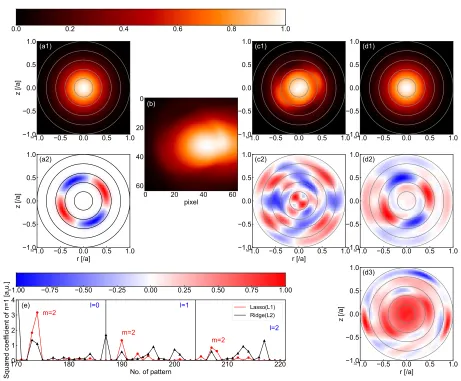
When the emission profile is superposition of then= 0 component andn=1 component, which is closer to the real experiments, the performance of this reconstruction method is examined. Figure 6 (b) is the tangential emission image where both the toroidally constant (n =0) peaked emission profile of Fig. 6 (a1) and the magnetic island like structure of the Fig. 6 (a2) (m/n =2/1 type) are assumed. Here, m and n are the poloidal and toroidal mode number, respectively.
Reconstructed image with one camera data is shown in Fig. 6 (c). The n = 0 mode and n = 1 mode is not separated well with this limited information. However, if the data from two camera systems observing at two toroidal locations (Fig. 4) are used, reconstructed images become more reasonable. Reconstruction of then=0 and n=1 component are shown in Fig. 6 (d1) and Fig. 6 (d2). Though the low amplitude noises can be seen in Fig. 6 (d2), fundamental characteristics of the n = 1 mode is ade-quately reconstructed.
L1 regularization is a key of this kind of reconstruc-tion. Fig. 6 (d3) is a reconstruction using L2 regularizareconstruc-tion. The noise is much larger especially in the core region of the image. One of the reasons of the merit of the L1 regulariza-tion is that less contributed components are neglected and not used. Fig. 6 (e) shows the amplitude of the coefficients for each component. Most of the coefficient for L1 regular-ization is zero and only the coefficients form=2 patterns are not zero and sufficiently large. Number of the coef-ficients equals to zero is 142/340 and 40/340 for L1 type and L2 type regularization, respectively. Mode structure withm=2 is thereby well enhanced in L1 type regulariza-tion results. The reconstrucregulariza-tion of limited informaregulariza-tion is thereby realized.
4. Summary
The performance of the series expansion method for the tomographic reconstruction are investigated. FB type pattern is capable for reconstruction with smaller number of patterns. However, the merit of the LE type that the only boundary information or the shape of the plasma is needed is also quite attractive and the performance of the LE type expansion is sufficient for this type of reconstruction study. The series expansion method applied for the tangentially viewing camera system is also promising from the numer-ical tests of the reconstruction. If two tangentially viewing camera systems located at two toroidal locations can be used, we can effectively separate n=0 component andn
Fig. 6 The emission profiles assumed are shown in Figs. (a1), (a2). Emission profile of exp(−(ρ/0.3)2) is assumed in (a1) and exp(−((ρ−
0.5)/0.05)2)∗cos(2θ+φ+0.25π) in (a2), respectively. Synthetic images from (a1) and (a2) are shown in (b). Reconstructed images
with one camera data ofn=0 andn=1 calculated by L1 regularization are shown in (c1) - (c2). Reconstructed images with two camera data are shown in (d1) and (d2). L2 regularization is used for (d3). Squared amplitude of coefficientsβiin L1 and L2 regularization are shown in (e).
using Saito’s method may also be a promising candidate for the reconstruction of the tangentially viewing images judging from the results of this article.
Acknowledgments
One of the authors (S. O.) is grateful for the discussion with Prof. Furukawa and Prof. Yokoyama. This work is partly supported by the by the Ministry of Education, Sci-ence, Sports and Culture Grant-in-Aid for Scientific Re-search 26249144. It is also supported by Japan/U. S. Co-operation in Fusion Research and Development.
[1] L.C. Ingessonet al., Fusion Sci. Technol.53, 528 (2008). [2] Y. Nagayama, J. Appl. Phys.62, 2702 (1987).
[3] T. Obiki et al., Plasma Phys. Control. Fusion 42, 1151
(2000).
[4] S. Yamamotoet al., Nucl. Fusion57, 126065 (2017). [5] N. Iwamaet al., Appl. Phys. Lett.54, 502 (1989). [6] S. Purohitet al., Rev. Sci. Instrum.89, 10G102 (2018). [7] S.P. Hirshman and J.C. Whitson, Phys. Fluids 26, 3553
(1983).
[8] N. Saito, J. Plasma Fusion Res.92, 905 (2016). [9] N. Saito, Appl. Comput. Harm. Anal.25, 68 (2008). [10] W.N. Van Wieringen, “Lecture notes on ridge regression”,
arXiv:1509.09169 (2018).
[11] S. Ohdachiet al., Rev. Sci. Instrum.74, 2136 (2003). [12] M.W. Shaferet al., Rev. Sci. Instrum.81, 10E534 (2010). [13] M.W. Shafer et al., “Observation of Multiple Helicity
Mode-Resonant Locking Leading to a Disruption on DIII-D”, in proc of IAEA-FEC conf. Oct. 21-27, Ahmedabad, In-dia, EX/P6-24.