DTU Wind Energy, Technical University of Denmark, Roskilde, Denmark Correspondence:Alfredo Peña ([email protected])
Received: 31 August 2018 – Discussion started: 21 September 2018
Revised: 17 December 2018 – Accepted: 20 December 2018 – Published: 15 January 2019
Abstract. We propose a method to assess the accuracy of atmospheric turbulence measurements performed by sonic anemometers and test it by analysis of measurements from two commonly used sonic anemometers, a Metek USA-1 and a Campbell CSAT3, at two locations in Denmark. The method relies on the estimation of the ratio of the vertical to the along-wind velocity power spectrum within the inertial subrange and does not require the use of another measure-ment as reference. When we correct the USA-1 to account for three-dimensional flow-distortion effects, as recommended by Metek GmbH, the ratio is very close to 4/3 as expected from Kolmogorov’s hypothesis, whereas non-corrected data show a ratio close to 1. For the CSAT3, non-corrected data show a ratio close to 1.1 for the two sites and for wind di-rections where the instrument is not directly affected by the mast. After applying a previously suggested flow-distortion correction, the ratio increases up to≈1.2, implying that the effect of flow distortion in this instrument is still not properly accounted for.
1 Introduction
Accurate observations of atmospheric flow velocities, turbu-lence, and turbulence fluxes are critical for our understanding of all physical processes that occur in the atmospheric bound-ary layer and for the improvement of atmospheric model-ing. Examples of intensely researched applications of turbu-lent fluxes include the closure of the surface energy balance (Foken, 2008), as well as the estimation of the carbon bal-ance based on eddy-covaribal-ance observations, in which a very small systematic error can have a significant effect on the yearly carbon budget (Ibrom et al., 2007). Other applications include wind-power meteorology: turbulence is an important design parameter for wind turbines as the turbine loads are
directly related to the velocity variances, and turbulence mea-surements are therefore needed to find out whether a wind turbine can withstand the local flow conditions (Mücke et al., 2011; Dimitrov et al., 2015).
Our current understanding of atmospheric turbulence is, to a high degree, based on measurements performed with three-dimensional sonic anemometers deployed on meteorologi-cal towers. However, sonic anemometer measurements suf-fer from flow distortion due to the effects of both the struc-ture(s) where the anemometer is mounted on, i.e., booms, clamps, and the bulk of the mast itself (e.g., Dyer, 1981; Mc-Caffrey et al., 2017), and the anemometer itself. The latter effect has been recognized as a limitation for the accuracy of sonic anemometer observations for several decades (Wyn-gaard, 1981; Zhang et al., 1986; Grelle and Lindroth, 1994; van der Molen et al., 2004; Horst et al., 2015).
an-gles. Whereas surface sensible heat flux observations taken over forest increased by 4 % using the calibration scheme by Grelle and Lindroth (1994), the calibration scheme by van der Molen et al. (2004) resulted in sensible heat flux in-creases of 15 % for a different forested site. For the USA-1 (or its more modern version the uSonic3) sonic anemometer from Metek GmbH, Hamburg, Germany, two-dimensional and three-dimensional flow-distortion corrections were pro-vided by Metek GmbH (2004) (hereafter M04). They are based on wind-tunnel observations for a number of azimuths and tilt angles.
Högström and Smedman (2004) documented an intercom-parison between hot-film anemometers and Gill Solent R2 and R3 sonic anemometers. Both types of instruments were calibrated in a wind tunnel and subsequently intercompared in full-scale experiments. Whereas the hot-film anemome-ters retained their precision from the calibration, that of the sonic anemometers deteriorated in the field tests. Högström and Smedman (2004) argued that this difference could be ex-plained by the effect of atmospheric turbulence and, hence, that wind-tunnel-based calibrations may not be valid.
Another method for testing the precision and accuracy of sonic anemometers is to mount different brands closely and study the agreement between their turbulence measurements (e.g., Mauder et al., 2007; Kochendorfer et al., 2012). The challenge with this method is the difficulty to objectively determine which of the sonic anemometers measures best. Also, if agreement is found, this could be due to a similar error.
A third variant for assessing sonic anemometer perfor-mance is by comparing several of the same brand by mount-ing them at different tilts (Meyers and Heuer, 2006; Kochen-dorfer et al., 2012; Nakai and Shimoyama, 2012) and az-imuths (Kaimal et al., 1990). Nakai and Shimoyama (2012) used five WindMaster sonic anemometers mounted at differ-ent angles relative to each other and deduced flow-distortion correction schemes based on the anemometers’ different re-sponses as a function of both tilt and azimuth angles. Since the geometry of the WindMaster is identical to that of the Solent R2 and R3, the resulting flow-distortion correction scheme could be compared to that of van der Molen et al. (2004). The new scheme by Nakai and Shimoyama (2012) pointed to slightly higher increases in the turbulent fluxes than that by van der Molen et al. (2004). Kochendorfer et al. (2012) used three sonic anemometers by R. M. Young, and studied the observations of the vertical wind speed over a wide range of azimuth and tilt angles. They found that for their sites, the vertical wind speed was underestimated by ≈11 %, and when applying their derived corrections, the heat fluxes increased by 9 %–13 %. Whereas this method avoids the potential problems associated with quasi-laminar wind-tunnel calibrations, the accuracy of the correction can-not be better than the accuracy of the instrument chosen as the reference. Also, it is hard to evaluate whether the some-what “busy” setup with several sonic anemometers in a small
area could lead to additional and larger flow distortions than those using a single sonic anemometer.
Several combinations of the three different methods out-lined above (wind-tunnel calibration, comparison of differ-ent brands of sonic anemometers, and tilting sonic anemome-ters of the same brand relative to each other) have also been demonstrated. Using four CSAT3 sonic anemometers and one ATI sonic anemometer, where two of the CSAT3 instru-ments were rotated 90◦, Frank et al. (2013) showed that the CSAT3 underestimated the vertical velocities, which led to an underestimation of the sensible heat flux of about 10 %. Horst et al. (2015) (hereafter H15) used a combination of all three of the methods to derive a flow-distortion correction for the CSAT3. Their correction, when applied to sensible heat flux data taken over an orchard canopy, showed a more modest effect closer to 5 %. Based on the same data as those in Frank et al. (2013), Frank et al. (2016) demonstrated the use of a Bayesian model to estimate the most likely flow-distortion correction scheme of the CSAT3 and found a 10 % increase in vertical velocities and sensible heat flux as well. Huq et al. (2017) presented a novel approach for estimating the accuracy of the CSAT3 by using numerical simulations. The results of the study pointed to flow-distortion errors of similar magnitude as those in H15. The discrepancies in the findings of the previous studies foster the debate on the mag-nitude of the CSAT3 flow-distortion correction. Given the key role that sonic anemometers have in the field of exper-imental micrometeorology, it is of great importance to find objective standards by which accuracy and precision can be evaluated.
The aim of the current study is two-fold. First we introduce a new method for evaluating sonic anemometer accuracy, and second, we evaluate the effect of flow-distortion corrections for two different sonic anemometers using this method. The two sonic anemometers are the USA-1, for which we apply the manufacturer’s flow-distortion correction, which is based on wind-tunnel measurements, and the CSAT3, for which we apply the correction by H15. To our knowledge, the method, which is based on the relation between the velocity spectra within the inertial subrange, has not been used previously for diagnosing sonic anemometer accuracy.
2 Background and methods
We first start by introducing the expected relations between velocity spectra within the inertial subrange in Sect. 2.1 and later introduce the flow corrections commonly used for sonic anemometers measurements in Sect. 2.2.
2.1 Inertial subrange
wherek1is the along-wind wavenumber, andαis the univer-sal Kolmogorov constant (≈0.5). Statistical isotropy of the second order means that no second-order statistics change if the coordinate system is rotated in any way. This would im-ply that the variances of the three velocity components would be identical and the covariances would be zero. But we can say that turbulence is locally isotropic within the inertial sub-range, which means that within that range all one-point cross-spectra between different velocity components approach zero faster than the velocity-component spectra. For example, the cross-spectrum betweenuandw, wherewis the vertical ve-locity component, decreases likek1−7/3, which is more rapid thanFu and the bulk of the momentum fluxhu0w0i, where
the prime indicates fluctuations, is located at a wavenumber lower than the inertial subrange. Due to incompressibility and isotropy, the velocity power spectra follow the relation (Pope, 2000),
Fw(k1)=Fv(k1)= 4
3Fu(k1), (2)
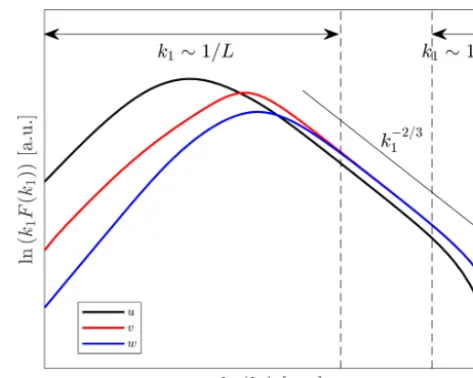
wherevis the cross velocity component. Figure 1 illustrates idealized velocity spectra showing the spectral regions, the behavior of each velocity component, and the relations in the inertial subrange. It is important to note that Eq. (2) is only an asymptotic relation valid for 1/Lk11/ηwhere Lis an outer scale of the turbulence, for example, the most energy-containing scales, andη= ν3/ε1/4, whereηis the Kolmogorov length scale andνthe kinematic viscosity. Also important is thatηis much smaller than the distance between transducers of a typical sonic anemometer (also known as path length), so viscosity is not important for the fluctuations measured by such an instrument.
2.2 Corrections to sonic anemometer measurements 2.2.1 Path-length averaging correction
For observations taken near the surface or during stable atmospheric conditions, the path length p over which the wind field is averaged may be a significant fraction of the length scale of the turbulence. A measured velocity power spectrum can therefore show a reduction of magnitude in the inertial subrange. Using similar methods as in Kaimal
Figure 1.Idealized atmospheric velocity spectra showing the spec-tral regions and the relations in the inertial subrange (indicated within the vertical dashed lines). Notice that the spectra in theyaxis are premultiplied byk1and so the spectral slope is−2/3 instead of −5/3 as in Eq. (1).
et al. (1968), Horst and Oncley (2006) (hereafter H06) calcu-lated how path-length averaging influences sonic anemome-ter measurements for the geometries of the CSAT3 and Gill R3 sonic anemometers. The path-length averaging errors are expressed as transfer functions for each velocity component and depend onk1p. Here, we implement the results by H06 using the transfer functions for each of the velocity compo-nents by means of interpolation of tabular values to observed k1p values. The tabular values for the CSAT3 are listed in H06, Table BI, Appendix B. Since the USA-1 has the same geometry as the Gill R3, the values in Table BII, Appendix B in H06 can be applied to the former instrument. It turns out that the effect of path-length averaging on the three velocity components is different for both the CSAT3 and Gill R3 ge-ometries. Fork1<1/p, which is the most relevant range for this investigation, theucomponent is more attenuated than thevandwcomponents.
2.2.2 Flow-distortion correction for the CSAT3 sonic anemometer
We implement the scheme by H15, which is based on that by Wyngaard and Zhang (1985) and calibrated through wind tunnel observations. The procedure has the following steps:
1. calculation of the length of the instantaneous wind vec-torS=px2+y2+z2, wherex,y, andzare the raw velocity components in the instrument’s coordinate sys-tem;
3. calculation of the angle between the wind vector and each of the paths (subindex p), θi=arccos(up,i/S),
wherei=1–3 denote paths 1–3, andup,i the projection
of the velocity component on each path;
4. correction (subindex c) of transducer shadowing up,i,c=up,i/(0.84+0.16 sinθi); and
5. a final rotation of the corrected velocities back to a Cartesian coordinate system.
2.2.3 Flow-distortion corrections for the Metek USA-1 sonic anemometer
There are two types of flow corrections available for the USA-1. The first one is a two-dimensional (2-D) correction that takes into account the azimuth angle and, the second, a three-dimensional (3-D) correction accounting for the tilt as well. Both are suggested by M04. The 2-D-corrected veloci-ties are
x2-D=xδ, (3)
y2-D=yδ, (4)
z2-D=z+0.031Ur[sin(3α)−1], (5)
whereδ=1.00+0.015 sin(3α+π/6),Ur=δ x2+y2 1/2
, andα= −atan2(y, x). The 3-D correction is applied through look-up tables (LUTs) derived from wind-tunnel measure-ments. Defining the instantaneous horizontal wind vector as Sh= x2+y2
1/2
, and the azimuth and tilt angles as α=atan2(−y,−x)andφ= −atan2(z,Sh), the velocity, az-imuth, and tilt are corrected as
V3-D=nc(α, φ)S, (6)
α3-D=α+αc(α, φ), (7)
φ3-D=φ+φc(α, φ), (8)
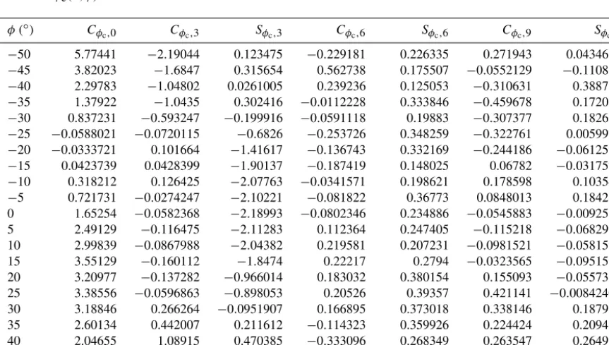
where nc(α, φ), αc(α, φ), and φc(α, φ) are α- and φ-dependent correction factors (note that there is a typo inV3-D in M04), which are computed through Fourier series with co-efficientsCf,i(φ)andSf,i(φ)that are provided in the LUTs,
fc(α, φ)= X
i=0,3,6,9
Cfc,i(φ)cos(iα)+Sfc,i(φ)sin(iα)
,
(9) wherefc(α, φ)is eithernc(α, φ),αc(α, φ), orφc(α, φ). The LUTs are not given in M04 and so we provide them in Ap-pendix A. The 3-D-corrected velocities are
x3-D= −V3-Dcosα3-Dcosφ3-D, (10) y3-D= −V3-Dsinα3-Dcosφ3-D, (11)
z3-D= −V3-Dsinφ3-D. (12)
3 Sites and instrumentation
Measurements were collected from sonic anemometers mounted on three meteorological masts at two sites in Den-mark: the Risø test site on the Zealand island and the Nør-rekær Enge wind farm on northern Jutland (see Fig. 2). The Risø test site is over a slightly undulating terrain with a mix of cropland, grassland, artificial land, and coast (the Roskilde Fjord coastline is≈250 m northwest of the turbine stands). The Nørrekær Enge wind farm is located≈350 m southeast of the water body Limfjorden over flat terrain with a mix of croplands and grasslands.
At the Risø test site, a CSAT3 was mounted at 6.4 m above ground level (a.g.l.) on a 2.5 m boom on a 15 m tall tower. The boom was oriented 14◦from the north. The tower was a triangular lattice structure with a side length of 0.4 m at the measurement height. The data acquisition unit was placed on the western leg of the tower, just below the boom. From the point of view of the mast, turbines were located within the direction sector 16–29◦.
Also at the Risø test site, but on a different mast, a USA-1 Basic was mounted at 16.5 m a.g.l. on a 2 m boom, which is oriented 10◦from the north, on a 54 m tall tower that is lo-cated west of the wind turbine stands. The tower is a square lattice structure 0.3 m wide from bottom to top. From the point of view of the mast, turbines are located within the di-rection sector 36–142◦.
At the Nørrekær Enge wind farm, a CSAT3 was mounted at 76 m a.g.l. on a 3.1 m boom, which is oriented 192.5◦from the north, on a 80 m mast that is located southeast of the row of wind turbines between stands 4 and 5, numbered from left to right. From the point of view of the mast, these two tur-bines are located within the direction sector 281–40◦. The closest turbine (4) is at 232 m and turbines are separated by 487 m. The mast is an equilateral triangular lattice structure with a width of 0.4 m at 80 m.
At all sites the sonic anemometers were mounted so that their north was aligned with the boom direction. Thus, wind directions are hereafter relative to the sonic anemometer ori-entation where 0◦is aligned with the boom. In Table 1, the specifications of the sonic anemometers at the two sites and the applied corrections are provided.
4 Data treatments
Figure 2.Locations of the sonic anemometer measurements. Wind turbines are indicated by black circles, masts with a CSAT3 by blue squares, and the mast with a USA-1 by a red square. Panel(a)shows the Risø test site and(b)the Nørrekær wind farm site. The color bar indicates the height above mean sea level in meters based on a digital surface elevation model (UTM32 WGS84).
Table 1.Sonic anemometer specifications for each measurement site including the types of flow-distortion (FD) and/or path-averaging (PA) corrections applied. Due to the height of the instrument at Nørrekær Enge, we did not apply a PA correction as the error should be negligible.
Site Sonic Height a.g.l. p Types of
anemometer (m) (mm) correction
Risø USA-1 16.5 175
none FD (M04)
PA (H06) and FD (M04)
Risø CSAT3 6.4 115
none FD(H15)
PA (H06) and FD (H15)
Nørrekær Enge CSAT3 76.0 115 none
FD (H15)
4.1 USA-1 at the Risø test site
The USA-1 measurements at Risø were sampled at 20 Hz. We used (a total of 25 401) 10 min time series of measure-ments conducted in 2014 in order to have sufficient data cov-ering all directions. We did all spectra calculations on each the raw (non-corrected data), the 2-D-, and 3-D-corrected data. We also applied the path-length averaging correction by H06 to the 3-D-corrected data.
4.2 CSAT3 at the Risø test site
The CSAT3 measurements at Risø were taken between November 2013 and mid-January 2014, and sampled at 60 Hz. For the analysis, it was required that all recorded ve-locities had the manufacturer’s quality signal equal to zero. Two velocity corrections were performed: the path-length av-eraging (H06) and the flow-distortion correction suggested by H15. After the quality signal filter, the amount of 10 min time series left were 2720.
4.3 CSAT3 at the Nørrekær Enge wind farm
The CSAT3 measurements at Nørrekær Enge were sampled at 10 Hz. We used (a total of 27 837) 10 min time series of measurements conducted in 2015, when the manufacturer’s quality signal was equal to zero and no precipitation was recorded by a rain gauge on the mast. We also applied the flow-distortion correction suggested by H15.
5 Results
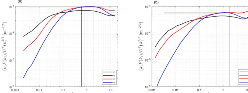
Figure 3.Ensemble-averaged, 3-D-corrected velocity spectra by the USA-1 at the Risø test site at 16.5 m for two directions intervals: one parallel 0±10◦(a)and another perpendicular 90±10◦(b)to the boom. A 0◦polynomial (c) was fit to the normalizedwspectra within the wavenumber range indicated by black vertical lines.
spectra were multiplied byk12/3(in contrast to the idealized wavenumber premultiplied spectra in Fig. 1) so that the iner-tial subrange can be distinguished as a flat region.
Second, for the selected wavenumber range, the velocity spectra ratios were computed for each 10 min sample and the statistics of these ratios were calculated for a wind direction range where the influence of the mast should be the lowest and incorporated in Table 2. We also show all 10 min veloc-ity spectra ratios as a function of direction (with and with-out flow corrections). For the specific case of the USA-1, we show the ratios of the velocity variances as function of direc-tion as well.
Further, to assess whether or not within the selected wavenumber range the velocity spectra conformed to the ex-pected behavior within the inertial subrange, we also filtered out “poorly” behaved spectra (e.g., from those winds affected by wind turbine wakes) by assuring that within the selected wavenumber range, both the slope of the w velocity spec-trum was −5/3±0.003 and |Fuw/
√
FuFw|<0.02 (i.e., a
uw co-covariance test narrowing for isotropy, see Sect. 2.1) for each 10 min sample. The slope was computed by fit-ting a 0◦polynomial to the normalizedwspectra within the selected wavenumber range. We call these two latter tests “sharpened” criteria in Table 2.
5.1 USA-1 at the Risø test site
Figure 3 shows two examples of 3-D-corrected velocity spec-tra, ensemble-averaged over two direction intervals for mea-surements of the USA-1 at the Risø test site. It is seen that for both direction intervals, the region in which the wvelocity spectrum becomes flat is within the same wavenumber range (0.5 m−1≤k1≤1.8 m−1). It is also observed that the spectra of the directions parallel to the sonic orientation have higher power spectral density than those of the directions perpen-dicular because for the latter, the spectra are influenced by
the fjord. Thus, we assumed at first that each 10 min spec-trum can be analyzed within the same range, irrespective of the wind conditions; this assumption is later tested using the sharpened criteria.
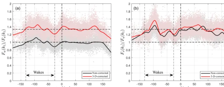
Figure 4a shows the w tou spectra ratio for each non-corrected and 3-D-non-corrected 10 min. It is clearly seen that the non-corrected data approach a ratio close to 1, whereas the 3-D-corrected data approach 4/3. Figure 4b shows thev touspectra ratio for each non-corrected and 3-D-corrected 10 min. It is shown that both sets of data approach a ratio close to 4/3, although the 3-D correction seems to generally increase the ratio. Theuandvspectra did not change much after the 3-D correction (not shown). Table 2 provides the computed velocity spectra ratios within the inertial subrange for the direction interval where there was no direct influence by the mast or winds were not affected by turbine wakes and for each the non-corrected measurements, the 3-D corrected, and the path-length averaging- and 3-D-corrected measure-ments. It is important to note that for all correction types, thevtouspectra ratio is close to 4/3 and that by applying the sharpened criteria, the statistics on both spectra ratios did not change significantly. The effect of path-length averaging (H06) on the spectra ratios was opposite to that of the 3-D correction but rather small.
Figure 4.Velocity spectra ratios by the USA-1 at the Risø test site as function of wind direction.(a)wtouvelocity and(b)vtouvelocity spectra ratios for the non- and 3-D-corrected data. Each 10 min ratio is shown in markers and the solid lines show a loess fit of the scatter. The thick dashed vertical line indicates the 0◦direction, the thin dashed vertical lines indicate the sector with possible turbine wakes, and two dashed horizontal lines the values 1 and 4/3. The standard error of the fit to the 3-D-correctedwtouvelocity spectra ratios is within 0.0020–0.0031.
Table 2.Computed velocity spectra ratios within the inertial subrange for the direction range within±120◦and excluding directions possibly affected by turbine wakes. The mean value is given±1 standard deviation.
Site Sonic anemometer Correction type Sharpened criteria Fw(k1)/Fu(k1) Fv(k1)/Fu(k1)
Risø USA-1 none no 0.984±0.089 1.322±0.127
Risø USA-1 FD (M04) no 1.343±0.125 1.362±0.129
Risø USA-1 FD (M04) and PA (H06) no 1.328±0.124 1.346±0.128
Risø USA-1 FD (M04) and PA (H06) yes 1.336±0.123 1.354±0.135
Risø CSAT3 none no 1.132±0.065 1.344±0.091
Risø CSAT3 FD (H15) no 1.194±0.070 1.373±0.093
Risø CSAT3 FD (H15) and PA (H06) no 1.155±0.068 1.320±0.089
Risø CSAT3 FD (H15) and PA (H06) yes 1.173±0.070 1.312±0.084
Nørrekær Enge CSAT3 none no 1.070±0.220 1.319±0.311
Nørrekær Enge CSAT3 FD (H15) no 1.127±0.237 1.340±0.327
Nørrekær Enge CSAT3 FD (H15) yes 1.162±0.213 1.323±0.171
5.2 CSAT3 at the Risø test site
From the investigated sonic anemometers, the CSAT3 at Risø had the lowest measurement height. Since the velocity spec-tra scale with height, the inertial subrange was expected to be within a range of higher wavenumbers compared to those from the other two sonic anemometers. The wavenumber range at which the premultiplied velocity spectra from this sonic anemometer showed an approximately flat range is k1= [2,5]m−1(see Fig. 6). Such high wave numbers might be affected by white noise from the data acquisition itself. The upper limit of the k1 interval chosen for analysis was therefore limited, particularly for the u andv components (refer to Appendix B for an explanation of why each veloc-ity component is affected differently by noise), which caused the spectral slope to be greater than−5/3.
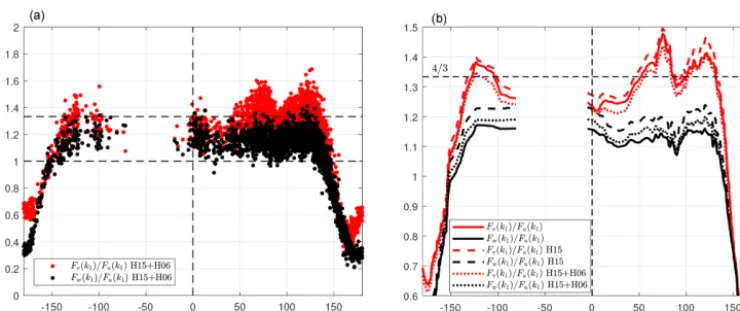
Figure 7 illustrates the computed velocity-component spectra ratios. Both Fw(k1)/Fu(k1) and Fv(k1)/Fu(k1)
showed very low values for absolute directions greater than ≈150◦. For directions more aligned to the boom, the ratios varied between 1.0 and 1.6 (Fig. 7a). For most of the direc-tional intervals, the ratioFv(k1)/Fu(k1)was clearly higher than theFw(k1)/Fu(k1)ratio. Due to the large difference in heights between this sonic anemometer and the hub height of the turbines in the site and because the closest turbine to the mast was not in operation during the acquisition of the sonic anemometer measurements, we judged that the wake effects are negligible for the computed ratios in Table 2. As shown in the table, the results for the mean velocity ratios were in-sensitive to the poor spectra filter. As for the USA-1 at Risø, for all correction types and criteria used, thev touspectra ratio was close to 4/3.
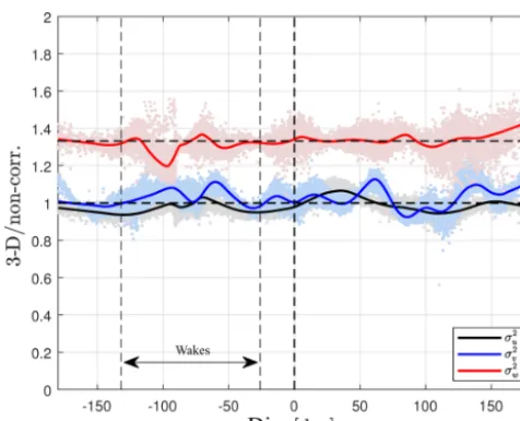
Figure 5.Ratios of the 3-D-corrected to the non-corrected velocity variances by the USA-1 at the Risø test site as function of the wind direction. Each 10 min ratio is shown in markers and the lines show a moving average of the scatter. Horizontal and vertical dashed lines as in Fig. 4.
It can be observed that the effect of path-length averaging (H06) was opposite to that of transducer shadowing (H15). As discussed before,Fu is attenuated more thanFvandFw
by path-length averaging in the inertial subrange. Therefore, when path-length averaging was accounted for, the ratios re-duced.
5.3 CSAT3 at the Nørrekær Enge wind farm
Figure 8 shows two examples of normalized velocity spectra, ensemble-averaged over two direction intervals for measure-ments of the CSAT3 at Nørrekær Enge as well as the polyno-mial fit within a chosen wavenumber range. The wavenum-ber range was limited to exclude noise apparent at higher wavenumbers (k1>1 m−1). Similar to the velocity spectra measured by the CSAT3 at the Risø test site, the w spec-trum closely followed the u spectrum and the v spectrum showed the highest spectral density within the inertial sub-range (0.38 m−1≤k1≤0.88 m−1).
Figure 9 shows thew andv tou spectra ratios for each 10 min. The result is very similar to that for the CSAT3 at the Risø test site where within a range of directions of ±150◦, thewtouspectra ratios were close to 1, whereas thevtou spectra ratios were close to 4/3. The boom and mast structure had a greater effect on the CSAT3 at the Nørrekær Enge wind farm than at the Risø site as expected due to the setup. For both sites, the effect of the boom and mast at directions close to±180◦ was very similar. In agreement with the findings using the CSAT3 at Risø (Sect. 5.2), the H15 correction in-creased both theFw(k1)/Fu(k1)andFv(k1)/Fu(k1)spectra ratios (particularly for the former) but not enough to reach the 4/3 value forFw(k1)/Fu(k1)(see Table 2). As for the
previous two cases, for all correction types and criteria, thev touspectra ratio was close to 4/3.
6 Discussion 6.1 Uncertainties
The aim of the spectral analysis displayed in Figs. 3, 6, and 8 was to find the optimal inertial subrange for each site and setup. A high-end limitation to this interval can be the pres-ence of white noise in the spectra, which would tend to re-duce the examined spectral ratios. For the velocity spectra at all three locations, we observe that the high-frequency wnoise is the lowest of the three velocity components and is proportionally lower for the CSAT3 than for the USA-1, which is consistent with its larger path elevation angle as explained theoretically in Appendix B. According to the theory, the noise in the v and u spectra should be identi-cal irrespective of the wind direction relative to the boom. The data showed deviations from this prediction. In addi-tion, for the Risø CSAT3 setup, numerous tests with regard to both wavenumber and frequency ranges were performed, resulting in only very slight changes to the results in Fig. 7 (not shown). Another test for the robustness of the results was performed by selecting only those spectra that showed close to perfect inertial subrange behavior within the selected wavenumber range (a close to−5/3 slope forFw(k1)and a lowuwco-covariance, see “Sharpened criteria” in Table 2), which increased the CSAT3 ratios at Risø by 0.6 %–1.6 % only.
The choice of thresholds for the sharpened criteria com-promised the amount of data left for the analysis; about 4 %, 25 %, and 1 % of the original amount of 10 min peri-ods for the USA-1 at Risø, CSAT3 at Risø, and the CSAT3 at Nørrekær Enge, respectively. The choice, however, did not change the velocity spectra ratios significantly. The softening of the values to, e.g., 0.03 and 0.2 for thewspectral slope and theuwco-covariance, respectively, resulted in a change of thewtouvelocity spectra ratio of≈0.6 % for the USA-1, ≈1.5 % for the CSAT3 at Risø, and≈0.8 % for the CSAT3 at Nørrekær Enge, only.
re-Figure 6.Similar to Fig. 3, but for the CSAT3 at the Risø test site. For the direction parallel to the boom(a), the average spectra were computed over 72 different 10 min samples, whereas for the directions perpendicular to the boom(b), the average was based on 453 different 10 min samples.
Figure 7.Velocity spectra ratios by the CSAT3 at the Risø test site as a function of wind direction for each 10 min period after applying the corrections in H15 and H06(a)and loess fits of the scatter(b). Horizontal and vertical dashed lines as in Fig. 4. The standard error of the fit to thewtouvelocity spectra ratios is within 0.0024–0.0072.
duction in the spectral ratio; therefore, we consider rotation-related errors to be of no importance.
6.2 Implications
We base our analysis on theoretical arguments about thew and v tou velocity spectral ratios, which should be equal to 4/3 within the inertial subrange. We find such ratios by applying the 3-D wind-tunnel-derived flow-distortion correc-tions to atmospheric velocity measurements performed with a USA-1 (Table 2), whereas applying a flow-distortion cor-rection to the CSAT3 results in ratios within the range 1.12– 1.19. If we assume that the discrepancy to 4/3 is due to re-maining uncorrected flow distortion and further, that flow distortion affects the observed frequencies equally, which is an assumption supported by the results presented in Huq et al. (2017), the imperfect ratios correspond directly to an underestimation in the velocity variances. Since our results
Figure 8.Similar to Fig. 3 but for the CSAT3 at the Nørrekær Enge wind farm.
Figure 9.CSAT3 velocity spectra ratios with wind direction at the Nørrekær Enge wind farm. Horizontal and vertical dashed lines as in Fig. 4. The standard error of the fit to thewtouvelocity spectra ratios is within 0.0038–0.0086 for the H15 correction.
Another clear result from the presented analyses concerns the difference between observed mast, boom, and instrument shadowing for the USA-1 and CSAT3; even from narrow masts and relatively long supporting booms, the mast in-fluence is more marked for the CSAT3 than for the USA-1. Whereas Foken (2008) recommended the use of sonic anemometers without a pole directly under the sonic mea-surement volume for atmospheric turbulence research, we stress here that this statement can at best be valid only for a limited wind direction interval. For anemometers mounted on bulky walk-up towers, the direction interval where data will be biased from the tower will likely be much larger. We further stress that a sonic anemometer that cannot reproduce a 4/3 ratio in the inertial subrange cannot be trusted to give accurate observations of all velocity components, provided
that an inertial subrange is clearly apparent. Despite a higher ratio of transducer diameter to path length, which is some-times used as a sonic anemometer quality marker, the USA-1, including the wind-tunnel-derived flow-distortion correction, therefore comes out better from our analysis.
6.3 Sonic anemometry quality assessments
We suggest that the spectral ratios of velocity components within the inertial subrange are a valuable addition to field tests and wind-tunnel calibrations. The advantage of the pre-sented method is that any sonic anemometer can be tested provided that inertial subrange characteristics are expected from the particular measurements. Unlike sonic anemometer intercomparisons, where ideal flat and uniform sites are pre-ferred (e.g., Mauder et al., 2007), the spectral ratio method did not seem to be sensitive to the spatial and flow hetero-geneity at the sites used here.
As mentioned above, a limitation to our method is that the accuracy of individual velocity components cannot be as-sessed; the 3-D-corrected observations from the USA-1, al-though almost perfect in terms of the 4/3 ratio, might still be inaccurate if all three velocity components are biased. Look-ing ahead, a reference for sonic anemometer measurements could be found in small-volume lidar anemometry (Abari et al., 2015), which is free of flow distortion.
6.4 Can wind-tunnel-based calibrations be trusted in atmospheric turbulence?
between sonic anemometer observations in wind tunnel and field tests in Högström and Smedman (2004) could also be that the velocities recorded by the early Gill sonic anemome-ters showed a marked temperature dependence (Mortensen and Højstrup, 1995).
≈33.33 % higher than those of the uncorrected measure-ments. For the CSAT3, which is commonly categorized as the sonic anemometer closest to being a distortion-free in-strument, the ratio of thewto theuvelocity spectra is≈1.1 without applying a flow-distortion correction. Using a previ-ously proposed flow-distortion correction, the ratios changed to≈1.15 on average, indicating that more work is needed to correctly quantify the flow distortion of this instrument. We propose to perform this type of analysis, in addition to field site intercomparisons and wind-tunnel calibrations, to assess the accuracy of sonic anemometer measurements. We also found that the influence of the mast, boom, and the in-strument itself was higher on the CSAT3 compared to the USA-1 measurements.
Appendix A: Metek USA-1 3-D flow-distortion corrections
Table A1.LUT forαc(α, φ).
φ(◦) Cαc,0 Cαc,3 Sαc,3 Cαc,6 Sαc,6 Cαc,9 Sαc,9
−50 −10.7681 1.83694 8.12521 1.76476 −0.120656 −0.31818 1.30896 −45 −7.57048 2.25939 4.22328 −0.0394204 −0.112215 −0.289935 1.99387 −40 −6.77725 0.293479 3.05333 −1.16341 0.433886 0.207458 1.05195 −35 −4.12528 2.24741 0.286582 −0.936084 0.205636 −0.399336 1.57736 −30 −2.00728 3.63124 −0.325198 −0.821254 0.236536 −0.303478 0.854497 −25 −3.1161 3.91749 −0.682098 −0.274558 0.401386 −0.531782 0.470723 −20 −1.73949 3.5685 −0.253107 0.0306742 0.236975 −0.290767 −0.224723 −15 −2.59966 2.7604 −0.425346 0.0557135 0.0392047 0.222439 −0.364683 −10 −1.80055 2.02108 −0.259729 0.161799 0.117651 0.513197 −0.0546757 −5 −1.02146 1.22626 −0.469781 −0.177656 0.402977 0.408776 0.513465 0 0.152354 0.208574 0.051986 −0.102825 0.480597 −0.0710578 0.354821 5 0.310938 −0.703761 −0.0131663 0.0877815 0.546872 −0.342846 0.176681 10 0.530836 −1.68132 −0.0487515 0.0553666 0.524018 −0.426562 −0.0908979 15 1.70881 −2.46858 −0.487399 0.207364 0.638065 −0.458377 −0.230826
20 2.38137 −3.37747 0.026278 0.0749961 0.759096 0.105791 0.0287425
25 3.81688 −4.13918 −0.690113 0.170455 0.474636 0.424845 0.232194 30 3.49414 −3.82687 −0.229292 0.54375 0.322097 0.387805 0.823967
35 4.1365 −3.22485 0.752425 0.755442 0.623119 0.250988 1.26713
40 5.04661 −2.53708 1.23398 0.623328 0.653175 −0.359131 1.43131
45 4.26165 −3.12817 2.61556 0.0450348 −0.330568 −0.34354 0.81789
Table A2.LUT forφc(α, φ).
φ(◦) Cφc,0 Cφc,3 Sφc,3 Cφc,6 Sφc,6 Cφc,9 Sφc,9
−50 5.77441 −2.19044 0.123475 −0.229181 0.226335 0.271943 0.0434668 −45 3.82023 −1.6847 0.315654 0.562738 0.175507 −0.0552129 −0.110839 −40 2.29783 −1.04802 0.0261005 0.239236 0.125053 −0.310631 0.388716 −35 1.37922 −1.0435 0.302416 −0.0112228 0.333846 −0.459678 0.172019 −30 0.837231 −0.593247 −0.199916 −0.0591118 0.19883 −0.307377 0.182622 −25 −0.0588021 −0.0720115 −0.6826 −0.253726 0.348259 −0.322761 0.0059973 −20 −0.0333721 0.101664 −1.41617 −0.136743 0.332169 −0.244186 −0.0612597 −15 0.0423739 0.0428399 −1.90137 −0.187419 0.148025 0.06782 −0.0317571 −10 0.318212 0.126425 −2.07763 −0.0341571 0.198621 0.178598 0.103543 −5 0.721731 −0.0274247 −2.10221 −0.081822 0.36773 0.0848013 0.184226 0 1.65254 −0.0582368 −2.18993 −0.0802346 0.234886 −0.0545883 −0.0092531 5 2.49129 −0.116475 −2.11283 0.112364 0.247405 −0.115218 −0.0682998 10 2.99839 −0.0867988 −2.04382 0.219581 0.207231 −0.0981521 −0.0581594 15 3.55129 −0.160112 −1.8474 0.22217 0.2794 −0.0323565 −0.0951596 20 3.20977 −0.137282 −0.966014 0.183032 0.380154 0.155093 −0.0557369 25 3.38556 −0.0596863 −0.898053 0.20526 0.39357 0.421141 −0.00842409
30 3.18846 0.266264 −0.0951907 0.166895 0.373018 0.338146 0.187917
35 2.60134 0.442007 0.211612 −0.114323 0.359926 0.224424 0.209482
40 2.04655 1.08915 0.470385 −0.333096 0.268349 0.263547 0.264963
Appendix B: Sonic anemometer noise
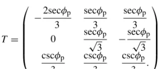
The transformation matrix to convert the three sonic path ve-locitiess=(s1, s2, s3), which are assumed positive from the lower to the upper acoustical transducer, to right-handed or-thogonal velocity components u=(u1, u2, u3)=(u, v, w), with u in the direction of the horizontal boom,v horizon-tal and transverse tou, andwin the vertical direction and positive upwards, is
T =
−2secφp 3
secφp 3
secφp 3 0 secφ√ p
3
−secφ√ p 3 cscφp 3 cscφp 3 cscφp 3 . , (B1)
whereφpis the path elevation angle, so
ui=Tijsj, (B2)
and we also assume the sonic anemometer paths to be ori-ented in the azimuthal direction like the CSAT3 or the USA-1.
Suppose now that the sonic anemometer signals are com-posed of uncorrelated, white noisehsisji =σs2δij, whereδis
the Kronecker delta symbol andσs2is the noise variance. The resulting noise on the orthogonal velocity components then becomes
huiuji = hTikskTj lsli =σs2TikδklTj l=σs2TikTj k
=σs2
2sec2φp
3 0 0
0 2sec
2φ p
3 0
0 0 csc
2φ p 3 . (B3)
Figure B1.The ratio of the noise level in the horizontal velocity components to the vertical one as a function of path elevation angle.
Acknowledgements. We would like to thank the technical support of the Test and Measurements section at DTU Wind Energy and in particular Søren W. Lund. Ebba Dellwik would like to thank the TrueWind project, which is funded by the Energy Technology Development and Demonstration Program (EUDP), Denmark, for financial support. Finally, we would like to thank Tom Horst for many inspiring discussions on flow-distortion corrections.
Edited by: Laura Bianco
Reviewed by: John Kochendorfer and one anonymous referee
References
Abari, C. F., Pedersen, A. T., Dellwik, E., and Mann, J.: Per-formance evaluation of an all-fiber image-reject homodyne co-herent Doppler wind lidar, Atmos. Meas. Tech., 8, 4145–4153, https://doi.org/10.5194/amt-8-4145-2015, 2015.
Dimitrov, N., Natarajan, A., and Kelly, M.: Model of wind shear conditional on turbulence and its impact on wind turbine loads, Wind Energ., 18, 1917–1931, 2015.
Dyer, A. J.: Flow distorsion by supporting structures, Boundary-Layer Meteorol., 20, 243–251, 1981.
Foken, T.: The Energy Balance Closure Problem: an Overview, Ecol. Appl., 18, 1351–1367, 2008.
Frank, J. M., Massman, W. J., and Ewers, B. E.: Underestimates of sensible heat flux due to vertical velocity measurement errors in non-orthogonal sonic anemometers, Agr. Forest Meteorol., 171– 172, 72–81, 2013.
Frank, J. M., Massman, W. J., and Ewers, B. E.: A Bayesian model to correct underestimated 3-D wind speeds from sonic anemometers increases turbulent components of the sur-face energy balance, Atmos. Meas. Tech., 9, 5933–5953, https://doi.org/10.5194/amt-9-5933-2016, 2016.
Grelle, A. and Lindroth, A.: Flow distortion by a Solent sonic anemometer: wind tunnel calibration and its assessment for flux measurements over forest and field, J. Atmos. Ocean. Tech., 11, 1529–1542, 1994.
Högström, U. and Smedman, A.-S.: Accuracy of sonic anemome-ters: laminar wind-tunnel calibrations compared to atmospheric in situ calibrations against a reference instrument, Bound.-Lay. Meteorol., 111, 33–54, 2004.
Horst, T. W. and Oncley, S. P.: Corrections to inertial-range power spectra measured by CSAT3 and Solent sonic anemometers,
Kaimal, J. C. and Finnigan, J. J.: Atmospheric boundary layer flows: Their structure and measurement, Oxford University Press, New York, 1994.
Kaimal, J. C., Wyngaard, J. C., and Haugen, D. A.: Deriving power spectra from a three-component sonic anemometer, J. Appl. Me-teor., 7, 827–837, 1968.
Kaimal, J. C., Gaynor, J. E., Zimmerman, H. A., and Zimmerman, G. A.: Minimizing flow distortion errors in a sonic anemometer, Bound.-Lay. Meteorol., 53, 103–115, 1990.
Kochendorfer, J., Meyers, T. P., Frank, J., Massman, W. J., and Heuer, M. W.: How well can we measure the vertical wind speed? Implication for fluxes of energy and mass, Bound.-Lay. Meteo-rol., 145, 383–398, 2012.
Kolmogorov, A. N.: The local structure of turbulence in incom-pressible viscous fluid for very large Reynolds number, Doklady ANSSSR, 30, 301–304, 1941.
Kraan, C. and Oost, W. A.: A new way of anemometer calibra-tion and its applicacalibra-tion to a sonic anemometer, J. Atmos. Ocean. Tech., 6, 516–524, 1989.
Mauder, M., Oncley, S. P., Vogt, R., Weidinger, T., Ribeiro, L., Bernhofer, C., Foken, T., Kohsiek, W., Bruin, H. A. R. D., and Liu, H.: The energy balance experiment EBEX-2000. Part II: intercomparison of eddy-covariance sensors and post-field data processing methods, Bound.-Lay. Meteorol., 123, 29–54, 2007. McCaffrey, K., Quelet, P. T., Choukulkar, A., Wilczak, J. M., Wolfe,
D. E., Oncley, S. P., Brewer, W. A., Debnath, M., Ashton, R., Iungo, G. V., and Lundquist, J. K.: Identification of tower-wake distortions using sonic anemometer and lidar measurements, At-mos. Meas. Tech., 10, 393–407, https://doi.org/10.5194/amt-10-393-2017, 2017.
Metek GmbH: Flow distortion correction for 3-d flows as measured by METEK’s ultrasonic anemometer USA-1, 2004.
Meyers, T. P. and Heuer, M.: A field methodology to evaluate sonic anemometer angle of attack errors, in: 27th Conference on Agr. Forest Meteorol., San Diego, California, 2006.
Mortensen, N. and Højstrup, J.: The Solent sonic – response and associated errors, Ninth Symposium on Meteorological Obser-vations and Instrumentation, 27–31 March 1995, Charlotte, NC, USA, 501–506, 1995.
Mortensen, N. G.: Flow-Response Characteristics of the Kaijo Denki Omni-Directional·Sonic Anemometer (TR-61B), Tech. rep., Forskningscenter Risoe, Denmark, 1994.
Nakai, T. and Shimoyama, K.: Ultrasonic anemometer angle of at-tack errors under turbulent conditions, Agr. Forest Meteorol., 162–163, 14–26, 2012.
Pope, S. B.: Turbulent Flows, Cambridge University Press, New York, 2000.
van der Molen, M. K., Gash, J. H. C., and Elbers, J. A.: Sonic anemometer (co)sine response and flux measurement: II. The ef-fect of introducting an angle of attack dependent calibration, Agr. Forest Meteorol., 122, 95–109, 2004.
Wilczak, J. M., Oncley, S. P., and Stage, S. A.: Sonic anemometer tilt correction algorithms, Bound.-Lay. Meteorol., 99, 127–150, 2001.
Wyngaard, J. C.: The effects of probe-induced flow distortion on atmospheric measurements, J. Appl. Meteorol., 20, 784–794, 1981.
Wyngaard, J. C. and Zhang, S.-F. F.: Transducer-Shadow Effects on Turbulence Spectra Measured by Sonic Anemometers, J. Atmos. Ocean. Tech., 2, 548–558, 1985.