https://doi.org/10.5194/amt-12-2155-2019 © Author(s) 2019. This work is distributed under the Creative Commons Attribution 4.0 License.
Intercomparison of MAX-DOAS vertical profile retrieval
algorithms: studies using synthetic data
Udo Frieß1, Steffen Beirle2, Leonardo Alvarado Bonilla3, Tim Bösch3, Martina M. Friedrich4, François Hendrick4, Ankie Piters5, Andreas Richter3, Michel van Roozendael4, Vladimir V. Rozanov3, Elena Spinei6,a, Jan-Lukas Tirpitz1, Tim Vlemmix5, Thomas Wagner2, and Yang Wang2
1Institute of Environmental Physics, University of Heidelberg, Heidelberg, Germany 2Max Planck Institute for Chemistry, Mainz, Germany
3Institute of Environmental Physics, University of Bremen, Bremen, Germany 4Royal Belgian Institute for Space Aeronomy (BIRA-IASB), Brussels, Belgium 5Royal Netherlands Meteorological Institute (KNMI), De Bilt, the Netherlands 6NASA-Goddard, Greenbelt, Maryland, USA
anow at: Virginia Tech, Blacksburg, Virginia, USA
Correspondence:Udo Frieß ([email protected]) Received: 3 December 2018 – Discussion started: 17 December 2018
Revised: 22 March 2019 – Accepted: 26 March 2019 – Published: 10 April 2019
Abstract. Multi-axis differential optical absorption spec-troscopy (MAX-DOAS) is a widely used measurement tech-nique for the detection of a variety of atmospheric trace gases. Using inverse modelling, the observation of trace gas column densities along different lines of sight enables the retrieval of aerosol and trace gas vertical profiles in the at-mospheric boundary layer using appropriate retrieval algo-rithms. In this study, the ability of eight profile retrieval al-gorithms to reconstruct vertical profiles is assessed on the basis of synthetic measurements. Five of the algorithms are based on the optimal estimation method, two on parametrised approaches, and one using an analytical approach without in-volving any radiative transfer modelling. The synthetic mea-surements consist of the median of simulated slant column densities of O4 at 360 and 477 nm, as well as of HCHO at 343 nm and NO2 at 477 nm, from seven datasets simulated by five different radiative transfer models. Simulations are performed for a combination of 10 trace gas and 11 aerosol profiles, as well as 11 elevation angles, three solar zenith, and three relative azimuth angles. Overall, the results from the different algorithms show moderate to good performance for the retrieval of vertical profiles, surface concentrations, and total columns. Except for some outliers, the root-mean-square difference between the true and retrieved state ranges
between (0.05–0.1) km−1 for aerosol extinction and (2.5– 5.0)×1010molec cm−3for HCHO and NO2concentrations.
1 Introduction
eleva-tion angles (EAs) ranging from near the horizon to the zenith, allow for the reconstruction of vertical profiles of the mea-sured trace gases and, using the oxygen collision complex O4 as a proxy for the light path, also of aerosol extinction. Us-ing suitable inverse models, trace gas and aerosol profiles can be retrieved in the lowermost≈2 km with a vertical resolu-tion of about 50–100 m at the surface and a lower resoluresolu-tion above. Up to four independent pieces of information can be retrieved.
Algorithms for the retrieval of vertical profiles from MAX-DOAS measurements can be separated into those that re-trieve vertical profiles on a finite vertical grid (usually with layers of 50–200 m in thickness) using the optimal estima-tion method (OEM) (Rodgers, 2000) and parametrised al-gorithms that use a small number of parameters (typically two to four) to describe the shape of the atmospheric profile. Parametrised algorithms are typically faster than OEM algo-rithms since they are usually based on precalculated look-up tables (LUTs), while OEM algorithms rely on online ra-diative transfer modelling (RTM). Being based on Bayesian statistics, OEM algorithms have the advantage of providing a thorough error analysis as well as a quantitative character-isation of the vertical resolution and the information content (Rodgers, 2000). However, the results of OEM algorithms critically depend on the appropriate choice of a priori con-straints, which are in many cases difficult to assess. In addi-tion to OEM and parametrised approaches, the present study also includes a fast algorithm developed by NASA, which relies only on geometrical considerations and only invokes radiative transfer modelling for a pure Rayleigh atmosphere. Testing the performance of algorithms for the retrieval of the atmospheric state using remote-sensing measurements on the basis of synthetic data is a method that has been widely used in the scientific community. In particular, nu-merous synthetic studies that investigated the performance of MAX-DOAS retrieval algorithms were published in the past (Wagner et al., 2004; Frieß et al., 2006; Hay, 2010; Vlemmix et al., 2011; Yilmaz, 2012; Hartl and Wenig, 2013; Holla, 2013; Zielcke, 2015). This paper presents the first in-tercomparison of eight state-of-the-art algorithms for the re-trieval of vertical profiles of aerosols and trace gases using synthetic MAX-DOAS measurements. Synthetic measure-ments have the advantage over ambient measuremeasure-ments that the true atmospheric state is exactly known, and thus a quan-titative comparison of true and retrieved atmospheric states is straightforward. This study is part of the Fiducial Refer-ence Measurements for Ground-Based DOAS Air-Quality Observations (FRM4DOAS) project funded by the Euro-pean Space Agency (see http://frm4doas.aeronomie.be, last access: 8 April 2019). One of the main objectives of this project is the development of a community algorithm for a harmonised near-real-time processing of MAX-DOAS data, including spectral analysis as well as the retrieval of tropo-spheric profiles of aerosols, HCHO and NO2, and strato-spheric NO2 profiles as well as total ozone columns. As
part of the FRM4DOAS project, the aim of the study pre-sented here has been the selection of suitable algorithms for the retrieval of tropospheric profiles to be integrated in the FRM4DOAS community algorithm.
The paper is structured as follows: Sect. 2 briefly de-scribes the inverse modelling theory and outlines the strategy for the intercomparison of the profile retrieval algorithms. A short description of the individual retrieval algorithms is provided in Sect. 3. The model scenarios and RTM settings are specified in Sect. 4. Slant column densities (SCDs) of NO2, HCHO, and the oxygen collision complex O4, simu-lated by the different RTMs serving as forward models for the retrieval algorithms, are compared in Sect. 5. Compar-isons of the quantities derived by the participating retrieval algorithms are presented in Sect. 6. These include averag-ing kernels from the OEM algorithms (Sect. 6.2), a posteri-ori modelled dSCDs (Sect. 6.3), vertical profiles (Sect. 6.4), total columns (Sect. 6.5), and aerosol extinctions and trace gas concentrations near the surface (Sect. 6.6). Finally, the numerical performance of the individual retrieval algorithms is assessed in Sect. 6.7.
2 Profile retrieval and intercomparison strategy In general, the retrieval of the atmospheric state (or the state of any physical system) by remote sensing is based on the observation of a finite number of quantities that represent the components of the measurement vectory, which is a function of the atmospheric statex,
y=F(x,b)+. (1)
Here, represents the measurement error. In the case of MAX-DOAS retrievals, the state vectorx consists of either aerosol extinction coefficients or trace gas concentrations in discrete atmospheric layers with a typical thickness of 50– 200 m. The measured quantities are differential slant col-umn densities (dSCDs) dS, usually the difference between the SCDSat a certain EAαand the SCD from a zenith sky measurement, observed along different lines of sight:
dS=S(α)−S(α=90◦), (2)
with the SCDSbeing the integrated concentration along the (average) light path through the atmosphere.
S=
Z
ρ(s)ds (3)
Here, ρ is the number density of the trace gas and s
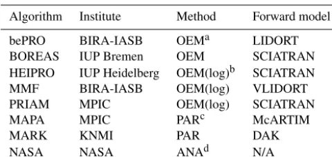
Table 1. MAX-DOAS retrieval algorithms participating in this study
Algorithm Institute Method Forward model
bePRO BIRA-IASB OEMa LIDORT BOREAS IUP Bremen OEM SCIATRAN HEIPRO IUP Heidelberg OEM(log)b SCIATRAN MMF BIRA-IASB OEM(log) VLIDORT PRIAM MPIC OEM(log) SCIATRAN MAPA MPIC PARc McARTIM
MARK KNMI PAR DAK
NASA NASA ANAd N/A
aOptimal estimation.bOEM(log): optimal estimation with logarithmic state vector. cParametrised retrieval.dAnalytical retrieval with RTM only for Rayleigh
atmosphere.
The aim of an inverse model is to provide an estimate of the atmospheric statexfor a given measurementy. However, in-verse problems are often poorly constrained, and the inin-verse of the forward model functionF−1, for which x=F−1(y)
either does not exist or the finite measurement errorleads to unstable estimates of the state vector.
To overcome these problems, MAX-DOAS retrieval algo-rithms make use of two different approaches. Retrieval al-gorithms using the well-known optimal estimation method (OEM) are based on a Bayesian approach (Rodgers, 2000). They introduce an a priori state vectorxa, together with an a priori covariance matrixSa, as an additional constraint. OEM algorithms are based on the minimisation of the following cost function:
χ2(x)=(y−F (x,b))TS−1(y−F (x,b))+(x−xa)T
S−a1(x−xa). (4)
HereSis the measurement covariance matrix, which, under
the assumption that the measurements are independent, is a matrix with the squares of the measurement errors (specified in Sect. 6.1 and Table 6) as diagonal elements and zero values elsewhere. The most probable (maximum a posteriori, MAP) estimatexˆ is then given as
ˆ
x=arg minχ2(x). (5)
The a priori constraintsxaandSarepresent the best knowl-edge of the atmospheric state before the measurement has been made, which can be derived, for example, from clima-tologies, but are often only based on rough estimates of the typical atmospheric conditions at the measurement site. The averaging kernel matrix (AVK)Aquantifies the sensitivity of the retrieved state to the true atmospheric state:
A=∂xˆ
∂x. (6)
The degrees of freedom for signal (DFS) ds=T r(A) quantify the number of independent pieces of information contained in the measurements. The jth row of the AVK represents the sensitivity of the retrieved amount in the at-mospheric layerj to the amount in all other layers, and the retrieved profile can be expressed by the true atmospheric profile, smoothed by the AVK according to
ˆ
x=xa+A(x−xa) . (7)
Parametrised retrieval algorithms do not explicitly intro-duce a priori constraints but overcome the problem that the state vector is poorly constrained by the measurements by representing the state vector as x=x(p), using only a small number (typically two to four) of parametersp=
(p1, . . ., pN) that describe quantities such as the total
col-umn, the layer thickness, and the shape of the profile. The cost function of parametrised algorithms is given as
χ2(p)=(y−F (x(p),b))TS−1(y−F (x(p),b)) (8) and the best estimate of the parameterspˆ is given as
ˆ
p=arg minχ2(p). (9)
OEM algorithms have the advantages that the approach, based on the well-established Bayesian statistics, is math-ematically stringent and that important parameters, such as the retrieval covariance matrix (separated into smoothing and noise covariance), AVK, and information content, can be readily derived. Parametrised algorithms are usually faster than OEM algorithms since the small number of parame-ters allows for the usage of precalculated LUTs, whereas OEM algorithms, with a larger number of state vector el-ements, usually perform radiative transfer calculations on-line. The calculation of the Jacobian matrix (weighting func-tion), which is required by OEM algorithms for the minimi-sation of the cost function, can be quite time consuming, es-pecially for non-linear problems, such as the aerosol profile retrieval. Parametrised algorithms have the disadvantage that the parametrisation limits the possible representations of the state vector to a certain subspace of the state vector space when characterising the state vector with a limited number of parameters. Conversely, OEM algorithms tend to be biased to the a priori, in particular in regions where the sensitivity to the atmospheric state is low.
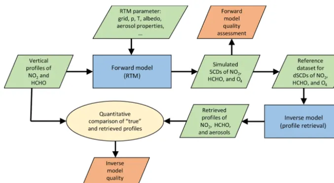
The overall strategy for the comparison of aerosol and trace gas vertical profiles from MAX-DOAS measurements within this study is depicted in Fig. 1. It consists of the fol-lowing steps.
and O4are performed for a variety of atmospheric sce-narios and viewing geometries as described in Sect. 4. In the following, these prescribed scenarios are referred to as the true atmospheric state, which is represented by the atmospheric state vectorx. This forward model intercomparison exercise allows for a quantitative com-parison of the individual RTMs on which the inversions are based (see Sect. 5).
2. The medians of the ensemble of dSCDs of HCHO, NO2 and O4from the different forward models derived from step 1 serve as a reference dataset that represents the measurement vectors for the different atmospheric sce-narios. This dataset was distributed among the partici-pants of this study and serves as input for the individual retrieval algorithms. This dataset is referred to below as the (synthetic) measurementsy.
3. The comparison of profilesxˆ retrieved by each partici-pant on the basis of the reference dataset with the true aerosol and trace gas profilesxallows for a quantitative assessment of the inverse models. The results of this in-tercomparison will be presented in Sect. 6.
4. Finally, a comparison of the numerical performance of the individual retrieval algorithms is performed (Sect. 6.7).
3 Retrieval algorithms
This section briefly describes the eight MAX-DOAS retrieval algorithms whose main features are listed in Table 1. Five of the algorithms are based on OEM, two on a parametrised ap-proach, and one (NASA) on an analytical approach without radiative transfer modelling. Each of the participants is free to decide on criteria for flagging particular retrieval results as invalid as described in the following subsections. If not stated otherwise, the comparison of retrieved quantities within this study is based on all data, without considering the validity flags.
3.1 The bePRO algorithm
The Belgian Profile (bePRO) OEM inversion algorithm was developed at the Royal Belgian Institute for Space Aeron-omy (BIRA-IASB) by Clémer et al. (2010). The forward model used in bePRO is the linearised discrete ordinate radia-tive transfer (LIDORT) code (Spurr et al., 2008). LIDORT is a multiple-scattering multilayer discrete ordinate scattering code with a simultaneous linearisation facility for the gen-eration of both radiances and analytical Jacobians (intensity partial derivatives with respect to any atmospheric or surface parameter). It uses the Green’s function method for solving the layer radiative transfer equations (RTEs), for both solar and thermal-emission sources. The analytical calculation of
the weighting functions allows near-real-time MAX-DOAS profile inversion without the use of precalculated weighting function LUTs. The bePRO algorithm uses a two-step ap-proach. First, the aerosol extinction vertical profiles are re-trieved for each MAX-DOAS scan from the corresponding measured O4dSCDs. Since it is a non-linear inversion prob-lem, the iterative OEM approach is used to minimise the cost function defined in Eq. (4). The standard aerosol re-trieval output includes the following parameters: aerosol ex-tinction profiles (per kilometre), aerosol optical depth, AVKs, smoothing and noise measurement error matrices, and O4 dSCDs calculated from the retrieved aerosol extinction pro-files using the forward modelF. In a second step, trace gas vertical profiles are retrieved using retrieved aerosol extinc-tion profiles as input for the calculaextinc-tion of the corresponding weighting functions. Since trace gases (except ozone) are op-tically thin absorbers, the OEM equation for the linear case is used (Rodgers, 2000).
The standard retrieval vertical grid used in bePRO is the following: 10 layers of 200 m in thickness starting from the altitude of the station, followed by two layers of 500 m in thickness and one layer of 1 km in thickness. This grid can be modified if needed.
A bePRO retrieval (aerosol or trace gas) is flagged as valid if the three following criteria are fulfilled: (1) the root mean square (RMS) of the difference between measured and simu-lated dSCDs<30 %, (2) DFS≥1, and (3) no negative value in the retrieved profile.
3.2 The BOREAS algorithms
The Bremen Optimal estimation REtrieval for Aerosols and trace gaseS (BOREAS) OEM algorithm (Bösch et al., 2018) developed at the Institute of Environmental Physics (IUP) Bremen uses the SCIAMACHY radiative transfer model (SCIATRAN) version 4.0.1 for the forward model calcu-lations and the SCIATRAN retrieval mode for the inver-sion of the aerosol extinction profile (Rozanov et al., 2014). However, since BOREAS is still under development, a pre-vious version of SCIATRAN was used (v3.8.12) together with a preliminary version of BOREAS within this study. SCIATRAN is run in BOREAS using the discrete ordinate mode with full multiple-scattering, full spherical geometry for single-scattering light and plane-parallel geometry for multiple-scattering light. Polarisation and rotational Raman scattering are usually not included in the forward model cal-culations. The weighting functions are calculated analyti-cally assuming an optianalyti-cally thin atmosphere.
pro-Figure 1.Flow diagram depicting the strategy for the retrieval algorithm intercomparison.
file. Again SCIATRAN in its full-spherical mode is applied. With the box air mass factors, the relation between the mea-surement and the absorber’s profile in the atmosphere can be expressed as a linear system, which is then solved by ap-plying the OEM to the measured slant columns and a priori profile information to retrieve trace gas profiles.
The profile retrieval is calculated based on SCIATRAN’s main grid and can be set by the user. The grid itself describes homogeneous layers around the grid points, with the excep-tion of the uppermost (lowermost) layer, which is considered to be half of the grid steps. BOREAS retrieval results are rou-tinely calculated on equidistant grid levels from the surface up to the maximum retrieval height. For each level, the re-trieved value is the average of the corresponding layer, e.g. in the case of the 200 m level, the altitude range from 100 to 300 m defines this specific layer. Two exceptions are the boundary levels, 0 and 4000 m, which cover only half the al-titude range compared to the other layers (0–100 and 3900– 4000 m). Since the grid was defined at the centre of the levels in this intercomparison study, BOREAS results were interpo-lated on these altitude values. Due to this interpolation, the lowest values in the submitted profiles are the interpolation between the retrieved surface value and the 200 m result.
Four different quality filters were applied. A profile is flagged as invalid if (1) the retrieved vertical column density is negative, (2) the profile contains more than 10 negative values, (3) the RMS between simulated and measured dSCD is larger than 2×10¹⁶molec cm−2for NO2and HCHO and 5×1043molec2cm−5for O4, and (4) the relative difference between the simulated and the measured dSCD for each line of sight is smaller than 5 %.
3.3 The HEIPRO algorithm
The Heidelberg Profile Retrieval Algorithm (HEIPRO) is an updated version of the algorithm already described in detail
in Frieß et al. (2006, 2011). It uses the SCIATRAN radiative transfer model version 2.1.5 (Rozanov et al., 2014) in dis-crete ordinate mode with full multiple-scattering, full spheri-cal geometry for single-scattering and plane-parallel geome-try for multiple-scattering light. The weighting functions for trace gases (box air mass factors) are calculated analytically; the weighting functions for aerosols are calculated using the finite difference method.
HEIPRO is based on OEM and retrieves the most prob-able state vector by minimising the cost function given by Eq. (4). The vertical extinction and aerosol profiles are rep-resented in the state vector as the logarithm of extinction and trace gas concentration, respectively. This has the advantages that (1) negative values, which cannot be processed by the RTM, are avoided, (2) the retrieval can reconstruct a larger range of atmospheric conditions, and (3) the retrieval is gen-erally more stable with less tendency to oscillations. As most MAX-DOAS retrieval algorithms, HEIPRO uses a two-step approach, where the aerosol extinction profile is retrieved in a first step using O4dSCDs as the measurement vector, and the trace gas profile is retrieved in a second step using the according trace gas dSCDs as the measurement vector, to-gether with the aerosol profile from the first step. The ra-diative transfer model SCIATRAN version 2.1.5 serves as a forward model for the retrieval.
No filtering of the HEIPRO data has been performed, and all profiles are flagged as valid.
3.4 The MMF algorithm
used. MMF can operate in linear or logarithmic state vector space. While different regularisation matrices are possible in the linear space, only Sa matrices of the form used in this study are currently tested in logarithmic mode. The results presented here were performed in logarithmic mode. MMF also uses a two-step approach, as outlined above in Sect. 3.3. Quantities such as aerosol single-scattering albedo, aerosol asymmetry factor, surface albedo, and temperature and pres-sure profiles can be supplied. In addition to the custom re-trieval grid, a simulation grid can be supplied. The algorithm has so far been applied in linear mode with Tikhonov regu-larisation for aerosol retrieval on an almost equal distance-in-pressure grid at UNAM (National Autonomous University of Mexico) for the retrieval of NO2profiles from four stations in the Mexico City area.
MMF flagging for this study was based on the mean of the ratio of the absolute value of the difference between mea-sured and simulated dSCD and the dSCD measurement error. The limit for flagging scans as invalid was 10.
3.5 The PRIAM algorithm
The OEM-based profile inversion algorithm of aerosol ex-tinction and trace gas concentration (PriAM) developed by the Anhui Institute of Optics and Fine Mechanics, Chinese Academy of Sciences (AIOFM, CAS), in cooperation with Max Planck Institute for Chemistry (MPIC), is introduced in Wang et al. (2013) and Frieß et al. (2016). A two-step in-version procedure is used in PriAM. In the first step, pro-files of aerosol extinction are retrieved from the O4dSCDs. The single-scattering albedo and asymmetry factor should be defined for the aerosol retrieval based on other auxil-iary measurements. Afterwards, profiles of volume mixing ratios (VMRs) of trace gases are retrieved from the respec-tive dSCDs in each MAX-DOAS EA sequence. The re-trieval problem is solved by the Levenberg–Marquardt mod-ified Gauss–Newton numerical iteration procedure (Leven-berg, 1944; Marquardt, 1963; Rodgers, 2000). PriAM uses the SCIATRAN 2.2 RTM (Rozanov et al., 2005) to calcu-late the weighting function and other simucalcu-lated quantities. To avoid meaningless negative values, the original aerosol ex-tinction and VMR of trace gases are transformed to the log-arithms of these quantities. Because of the conversion, it is necessary to use the nonlinear optimal inverse method to re-trieve the profiles of trace gases instead of the linear method. PriAM can retrieve trace gas and aerosol profiles on any ar-bitrary vertical grid.
3.6 The MAPA algorithm
The Mainz Profile Algorithm (MAPA) developed at the MPIC is a two-step algorithm based on a parametrised ap-proach. First, the aerosol profile is retrieved based on O4 dSCDs, and second, trace gas profiles are retrieved based on trace gas dSCDs and aerosol profiles from the first step.
The forward model is provided as a LUT, relating the profile parameters to O4and trace gas differential air mass factors (dAMFs) for given solar zenith angles (SZAs) and relative azimuth angles (RAAs) between the Sun and the instrument’s field of view. The LUT is calculated with the Monte Carlo Atmospheric Radiative Transfer Inversion Model (McAR-TIM) (v1), a full spherical Monte Carlo model without polar-isation (Deutschmann et al., 2011). Up to four parameters are determined independently: the integrated column (aerosol optical thickness, AOT; vertical column density, VCD), layer height, profile shape, and, in the case of aerosols, the O4 scaling factor (optional). The profile shape is described by the shape parameters, withs=1 representing a box profile,
s <1 representing a combined box profile with an exponen-tial profile on top (sdescribes the fraction of the box profile on the total profile), ands >1 representing elevated profiles. Previous versions of the parameter-based profile inver-sions, as described e.g. in Wagner et al. (2011), were based on a Levenberg–Marquardt least-squares algorithm. In MAPA (from v0.6 on), however, the profile retrieval is based on a Monte Carlo approach yielding an ensemble (instead of only one set) of best matching parameters. This approach is much faster (about 3 s per profile), accounts for correlations between the parameters, can deal with multiple minima, and allows the uncertainty of the resulting profiles to be deter-mined. MAPA is described in detail in Beirle et al. (2019).
MAPA uses RTM parameters for the LUT generation that slightly differ from those prescribed within this study (see Sect. 2), with a phase function asymmetry parameter of 0.68, aerosol single-scattering albedo of 0.95, and surface albedo of 0.05.
The MAPA flagging scheme is as follows. For each el-evation sequence, MAPA determines the parameter combi-nations yielding the best match of modelled and measured dSCDs, no matter how good this best match actually is. Thus, flagging is required in order to evaluate which MAPA results should be considered as meaningful and which not. MAPA provides a two-stage flagging scheme: moderate exceedance of the thresholds results in a warning, while large deviations raise an error. Flagging is based on different criteria. (1) The level of agreement between forward model and measurement compared to the dSCD error (for details see Beirle et al., 2019), (2) the consistency of column parameter within the Monte Carlo ensemble, and (3) the shape of the resulting profile, which is requested to be located in the lower tropo-sphere. In addition, scenes with high AOT (>2) are flagged as invalid. For RAA<15◦, even scenes with AOT>0.5 are
flagged. All flags are determined and stored individually and merged into one total flag defined as any of the flag criteria for both warnings and errors.
discussion on the impact of the a priori thresholds see Beirle et al. (2019).
3.7 The MARK algorithm
The MAX-DOAS retrieval KNMI (MARK) developed at the Royal Dutch Meteorological Institute (KNMI) is described in Vlemmix et al. (2011); Vlemmix et al. (2015a). It makes use of a profile shape parametrisation with just a few (two to four) free parameters. A LUT of differential slant col-umn simulations is produced by the Doubling-Adding KNMI (DAK) model (de Haan et al., 1987; Stammes et al., 1989). A standard least-squares algorithm is used to minimise the deviations between simulated and measured differential slant columns at the different EAs. Uncertainties in the parameters are estimated from the spread in the results of an ensemble approach in which the retrieval is performed multiple times with disturbed measured differential slant column densities, based on the DOAS retrieval uncertainties. For each individ-ual retrieval the aerosol profile is retrieved first, and the out-come is used in the trace gas retrieval. The ensemble retrieval is performed for four different parameterisations, and the re-ducedχ2distribution of the ensembles is used to make an a posteriori composite of the profile and its corresponding uncertainties. The fitted profile shape parameters are (1) the tropospheric column density (or AOT); (2) the top height of the mixing layer; (3) the shape parameter, which determines the linear increase or decrease in the mixing layer; and (4) the fraction of the total trace gas column density, which resides above the mixing layer.
MARK data are flagged as invalid if the variability in the AOT or the trace gas column within an ensemble is larger than 15 % of the value itself.
3.8 The NASA algorithm
The National Aeronautics and Space Administration (NASA) real-time algorithm was developed as a quick look algorithm that relies on the fact that atmospheric scatter-ing strongly affects DOAS-measured O4absorption (Spinei et al., 2019). Two separate approaches are used for aerosol and trace gas profile retrieval. The aerosol profile algorithm determines the layer aerosol extinction coefficients by com-paring measured ring and O4 absorption with ring and O4 absorption under pure Rayleigh conditions. Air mass fac-tors and ring absorption for the Rayleigh case are precal-culated using the VLIDORT v2.8 and LIDORT-LRRS v2.5 radiative transfer models, respectively (Spurr et al., 2008; Spurr, 2008), assuming the US standard atmosphere. Since ring simulations were not provided in this study, aerosol anal-ysis was performed only at 477 nm. O4dSCDs are corrected for SZA dependence. Equation (10) is the simplified equa-tion used in this study to calculate aerosol scattering extinc-tion coefficients at each layer for specific observaextinc-tion
geom-etry (EA and RAA)2. We also assume an aerosol single-scattering albedo ofωaer(λ)=1.
aer(λ, 2, ϑ )≈ τOnoaer
4,i −τ aer O4,i
1h , (10)
withτOaer
4,i andτ noaer
O4,i being the slant optical density with and without aerosols in the respective layeri,λdenoting wave-length, andϑ denoting the SZAs. The thickness1hof the respective layer is determined from the O4dSCDs using sim-ple trigonometry according to Eqs. (11) and (12), resulting in an atmosphere specific grid:
hi=
1SO4(αi)+VO4
nO4
·sinαi, (11)
1h=hi+1−hi, (12)
withSO4(αi)being the O4slant column density at elevation angleαi andVO4the O4vertical column density.
The maximum number of vertical layers is equal to the number of elevation angles. Profiles are considered invalid if fewer than four measurements are used in the profile calcu-lation, with all of the synthetic data analysed here satisfying this test. Within this study, an exponential profile decreasing to 0.01 % of the last altitude layer extinction coefficient at 4 km was added for consistency with the other algorithms. The resulting profile was then linearly interpolated on the common grid (200 m up to 4 km).
The trace gas profile retrieval does not rely on the aerosol retrieval. The trace gas VCDVgasis calculated first from the trace gas and O4dSCD measurements at 15◦EA,1S15–90
◦
gas :
Vgas=
1Sgas15–90◦ 1A15–90O ◦
4
, (13)
with the according O4dAMF1A15
◦−
90◦
gas calculated via
A15–90O ◦
4 =
1SO15–90◦
4
VO4
+1. (14)
Near-surface trace gas VMRsMgasare calculated by sim-ple extrapolation of trace gas and O4 dSCDs at 1 and 2 to 0◦ EA, yielding1S(α, λ)extrapolatedgas and1S(α, λ)
extrapolated
O4 ,
and by converting to the VMR using surface pressurepand temperatureT similar to Sinreich et al. (2013):
Mgas=
1S(α, λ)extrapolatedgas 1S(α, λ)extrapolatedO
4
·p·Na
R·T ·χ 2
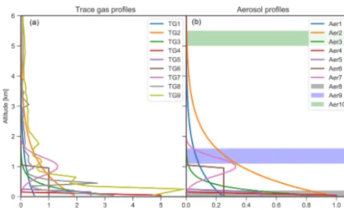
Figure 2.Trace gas number concentration(a)and aerosol extinction
(b)vertical profiles as input for the forward modelling of HCHO, NO2, and O4. The shaded areas in(b)indicate the location of fog and cloud layers with an extinction coefficient of 10 km−1. The properties of the individual profiles are described in Tables 2 and 3.
The rest of the profile VMR is calculated using O4 and trace gas dSCDs at multiple EAs. The layer altitude is calcu-lated similar to the aerosol case. The derived profile is then converted to partial columns and scaled by the total VCD. As in the aerosol case, the layer grid is condition specific and was adjusted to the common grid in this study.
4 Model scenarios and RTM settings
A first important step for the comparison of retrieval algo-rithms is the assessment of their capability to realistically simulate the underlying physical processes using appropri-ate forward models, which are in this case atmospheric ra-diative transfer models. This section describes the forward model parameters and atmospheric scenarios for the mod-elling of O4, NO2, and HCHO SCDs, while the comparison of forward modelled SCDs is presented in Sect. 5.
The model atmosphere for the forward calculations con-sists of 67 layers, with a resolution of 100 m at altitudes be-tween the surface and 4 km and a coarser resolution above. Note that the retrieval of extinction and trace gas profiles is performed on a coarser grid with 200 m resolution in the lowermost 4 km. The choice of a finer grid for the forward modelling than for the inverse modelling allows for the in-vestigation of the impact of sub-grid trace gas and aerosol variabilities on the retrieved profiles. For the forward mod-elling, a constant concentration within each layer has been implemented for the model calculations whenever possible.
The trace gas concentration and aerosol extinction pro-file scenarios for the forward modelling of HCHO, NO2 and O4 SCDs are shown in Fig. 2. The same set of trace gas profiles is assumed for both HCHO and NO2, in accor-dance with ambient measurements in mid-latitudes, where typical concentrations of both species are of the same
or-Table 2.Description of the trace gas profiles shown in Fig. 2. The VCD and the maximum number concentrationρmaxare given in units of 1015molec cm−2and 1011molec cm−3, respectively.
Description VCD ρmax
TG0 No trace gas 0.00 0.00
TG1 Exponential, 1 km scale height 5.00 0.48 TG2 Exponential, 1 km scale height 19.99 1.90 TG3 Exponential, 250 m scale height 9.93 3.27 TG4 Box profile, 100 m height 5.00 5.00 TG5 Box profile, 200 m height 5.00 2.50 TG6 Box profile, 1 km height 10.00 1.00 TG7 Gaussian at 1 km, 300 m FWHM 10.00 1.31 TG8 NO2balloon sonde (CINDI-2, 20160914) 17.73 3.30 TG9 NO2balloon sonde (CINDI-2, 20160921) 40.88 5.82
der of magnitude (e.g. Vlemmix et al., 2015b). For simplic-ity, it is assumed that aerosol extinction does not change with wavelength (Ångström exponent of zero). The model profiles are chosen in order to represent a large variety of different atmospheric conditions, including trace gas and aerosol free atmospheres as well as moderate to high trace gas and aerosol loads up to cloudy and foggy conditions. The shapes of the different profiles include near-surface box profiles, profiles exponentially decreasing with altitude, up-lifted profiles with a Gaussian shape, and profiles without trace gases and aerosols. Additionally, the trace gas scenar-ios include two NO2profiles measured with a balloon sonde during the CINDI-2 campaign conducted in the Netherlands in September 2016 (Kreher et al., 2019; see also http://www. tropomi.eu/data-products/cindi-2, last access: 8 April 2019). The aerosol scenarios include three extreme cases with an ex-tinction of 10 km−1located at the surface, as well as at alti-tudes around 1.3 and 5.25 km, representing fog and low-lying and high-lying clouds, respectively. In total, the scenarios in-clude 10 trace gas and 11 aerosol profiles whose features are listed in Tables 2 and 3, respectively. The forward calcula-tions of O4at 360 and 477 nm are performed for each of the 11 aerosol profiles. NO2and HCHO SCDs are simulated for each combination of aerosol and trace gas profiles, yielding in total 110 different trace gas scenarios.
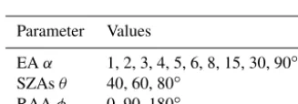
The viewing geometry for the forward model simulations is specified by the EAα, the SZAsθ, and the RAAφbetween the Sun and the viewing direction of the instrument. Simu-lations are performed using any combination of values for EA, SZAs, and RAA as listed in Table 4. The EA sequence, consisting of 10 angles between the horizon and zenith, is identical to the measurement sequence during the CINDI-2 campaign. Together with three SZAs and three RAA values, this yields 90 different viewing geometries to be simulated for each model atmosphere.
Table 3. Description of the aerosol extinction profiles shown in Fig. 2. The maximum extinctionkmaxis given per kilometre.
Description AOT kmax
AER0 No aerosols 0.00 0.00 AER1 Exponential, 1 km scale height 0.25 0.24 AER2 Exponential, 1 km scale height 1.00 0.95 AER3 Exponential, 250 m scale height 0.25 0.82 AER4 Box profile, 100 m height 0.10 1.00 AER5 Box profile, 200 m height 0.10 0.50 AER6 Box profile, 1 km height 0.25 0.25 AER7 Gaussian at 1 km, 300 m FWHM 0.25 0.33 AER8 Box profile, 200 m height (fog) 2.00 10.00 AER9 Cloud between 1.1 and 1.6 km 5.00 10.00 AER10 Cloud between 5.0 and 5.5 km 5.00 10.00
Table 4. Viewing geometry for the model calculations. SCDs are simulated for each combination of EA, SZAs, and RAA.
Parameter Values
EAα 1, 2, 3, 4, 5, 6, 8, 15, 30, 90◦ SZAsθ 40, 60, 80◦
RAAφ 0, 90, 180◦
temperature and pressure derived from average ozone-sondes for the month of September from 2013 to 2015 in De Bilt, the Netherlands, as well as surface albedo, aerosol optical properties, and trace gas literature absorption cross sections. The aerosol scattering was parametrised using a Henyey– Greenstein phase function (Henyey and Greenstein, 1941) with the asymmetry parameter as listed in Table 5.
In total, all combinations of viewing geometries, aerosol profiles, and trace gas profiles yield 990 O4SCD simulations each at 360 and 477 nm and 9900 simulations for each of the trace gases NO2and HCHO.
5 Intercomparison of forward modelled SCDs
In this section, the ability of the forward models to realisti-cally simulate trace gas SCDs is assessed based on a com-parison of the individual simulations with the median of the SCDs from the different RTMs. The median SCDs also serve as a reference dataset and provide the synthetic mea-surements for the profile retrieval comparison presented in Sect. 6. Figure 3 shows the comparison of the simulated O4, NO2, and HCHO SCDs to the respective ensemble median. The respective parameters of a linear regression of forward modelled SCDs versus median SCDs are shown in Fig. 4. The SCDs simulated by most forward models agree under all conditions, with Pearson’s coefficients and slopes very close to unity (R >0.999 and 0.99<slope<1.001) for a regres-sion between SCDs from the individual models and the me-dian from all models. Exceptions are HEIPRO and PRIAM,
both using an older version of the SCIATRAN RTM (version 2.1) as the forward model. These models show deviations for the fog and cloud scenarios (AER8. . .AER10), the shallow box profile (AER4), and in the case of HEIPRO also for the exponential profile AER2 with a high AOT of 1. MAPA with McARTIM as the forward model yields significantly smaller slopes of 0.955 and 0.959 than the other models for O4 at 477 nm and for NO2, respectively. This is probably due to the different treatment of sphericity within the McARTIM model. Significant biases are found for MAPA–McARTIM and PRIAM–SCIATRAN for NO2and O4at 477 nm, as well as for HEIPRO–SCIATRAN for HCHO. Apart from possi-ble differences in the implementation and the approaches of the individual RTMs, some of the differences are likely due to the different representations of the trace gas and aerosol profiles on the prescribed vertical grid.
In summary, the SCDs simulated by the different radiative transfer models agree well under all conditions, as within previous RTM intercomparisons (e.g. Wagner et al., 2007). This implies that possible discrepancies in the retrieved trace gas and aerosol profiles are mainly caused by differences in the implementation of the retrieval algorithms, rather than by differences in the forward models.
6 Retrieval algorithm comparison
This section presents the results of the aerosol and trace gas retrieval algorithm intercomparison. Section 6.1 describes the measurement vectors, forward model parameters, and a priori constraints of the profile retrieval. An important diag-nostic tool is provided by the AVKs from the OEM algo-rithms, which quantify the sensitivity of the retrieval to the atmospheric state. AVKs and information content are dis-cussed in Sect. 6.2. The comparison of modelled and mea-sured dSCDs presented in Sect. 6.3 provides a measure for the level of convergence of the retrieval algorithms. Results of the intercomparison of vertical profiles, trace gas and aerosol total columns, and surface extinction and trace gas concentrations are presented in Sect. 6.4, 6.5, and 6.6, re-spectively. Finally, the computational speed of the retrieval algorithms is discussed in Sect. 6.7.
6.1 Retrieval settings
Table 5.RTM parameters for the radiative transfer modelling.
Parameter Value
Temperature and pressure profile Sept. 2013–2015 average from De Bilt ozone-sondes Surface albedo (Lambertian surface) 0.06
Aerosol single-scattering albedo 0.92 Aerosol phase function asymmetry parameter 0.68 Instrument height 0 km
O4absorption cross section 293 K (Thalman and Volkamer, 2013) NO2absorption cross section 298 K (Vandaele et al., 1998) HCHO absorption cross section 297 K (Meller and Moortgat, 2000)
Figure 3.Correlation of SCDs of O4(360 and 477 nm), HCHO, and NO2simulated by the different forward models with the corresponding median SCDs from all models. Colours indicate the underlying aerosol and trace gas profiles as denoted in the legend. For HCHO and NO2, results for all scenarios with different aerosol profiles are included.
Table 6.Assumed measurement errors of the O4, HCHO, and NO2 dSCDs, as well as total columns of the respective a priori profiles. Units for the errors are molec2cm−5for O4and molec cm−2for HCHO and NO2.
Species dSCD error λ A priori total column (nm)
O4 2×1041molec2cm−5 360 0.18 O4 2×1041molec2cm−5 477 0.18
HCHO 2×10¹⁵molec cm−2 343 8×10¹⁵molec cm−2 NO2 5×10¹⁴molec cm−2 460 9×10¹⁵molec cm−2
trace gas profiles, aerosol profiles, and solar geometry (SZAs and RAA).
Figure 4.Slope, intercept, regression coefficient, and root-mean-square difference (RMS) of the correlation between the SCDs from the individual forward models and the median SCDs from all models. RMS and intercept values are in units of 1043molec2cm−5for O4and 1017molec cm−2for HCHO and NO2.
Figure 5.The 360 nm aerosol AVKs. Each subplot shows the mean AVK over all SZAs and RAA for a specific aerosol scenario (columns) and retrieval algorithm (rows). Filled circles indicate the nominal altitude of the corresponding AVK plotted in the same colour. Colour-shaded areas (barely visible in most cases) indicate the standard deviation of the AVKs, i.e. the variation for different SZAs and RAA. Also shown are the DFS. AVKs stem from retrievals with noisy measurements (v1n).
scan with a typical duration of several minutes. The second noise component is of magnitude similar to the RMS differ-ences between dSCDs measured by more than 30 instruments during the CINDI-2 Campaign (Kreher et al., 2019).
Each participant performed retrievals with settings being as close as possible to the prescribed settings described be-low. The results based on noise-free and noisy dSCDs are la-belled “v1” and “v1n”, respectively. Each measurement vec-tor consists of O4, HCHO, or NO2dSCDs of a single EA
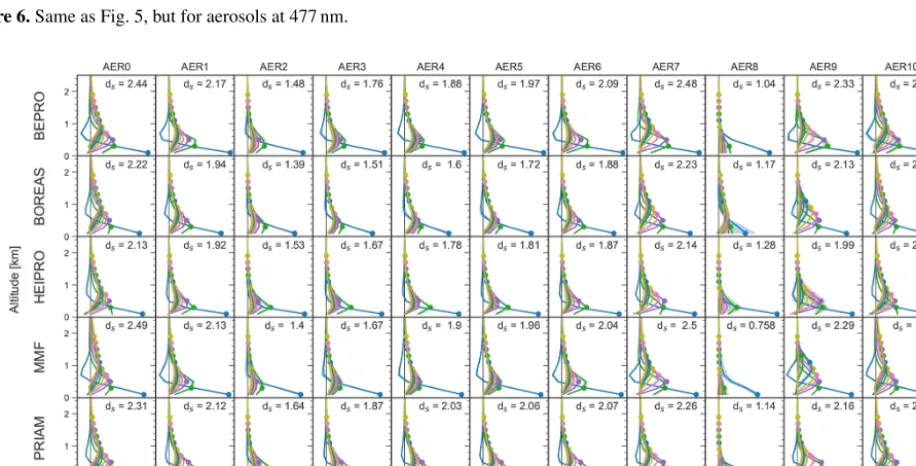
Figure 6.Same as Fig. 5, but for aerosols at 477 nm.
Figure 7.Same as Fig. 5, but for HCHO.
forward modelling. This choice allows for the investigation of the impact of sub-grid variations on the retrieval, in par-ticular in the case of scenarios TG4 and AER4 (100 m thick box profiles).
In contrast to the output of OEM algorithms, which di-rectly retrieve trace gas and aerosol profiles on this verti-cal grid, profiles from the parametrised algorithms are inter-polated onto the prescribed grid. The OEM algorithms use aerosol and trace gas a priori profiles exponentially decreas-ing with altitude with a scale height of 1 km, with a priori vertical columns for each species as listed in Table 6. The
Figure 8.Same as Fig. 5, but for NO2.
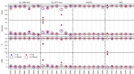
Figure 10. Slope, intercept, regression coefficient, and RMS of the dSCD correlation. Each of the circular symbols for the filtered data represents a pie chart that quantifies the fraction of data flagged as valid. RMS and intercept values are in units of 1043molec2cm−5for O4 and 1017molec cm−2for HCHO and NO2. Cloud and fog scenarios (AER8, AER9, AER10) are excluded from the regression analysis.
6.2 Comparison of averaging kernels
Figures 5, 6, 7, and 8 show the AVKs from the OEM al-gorithms for aerosols at 360 and 477 nm, HCHO, and NO2, respectively. The AVKs confirm that MAX-DOAS measure-ments yield only information on the lowermost ≈2 km of the atmosphere when using a zenith-sky reference spectrum from the same EA sequence. This is a result of the measure-ment geometry and, in the case of aerosols, also of the fact that the O4vertical distribution is heavily weighted to the sur-face. The DFS range fromds<0.5 during foggy conditions (AER8) tods>3 for aerosol-free atmospheres (AER0), with the information content being generally higher for aerosols than for trace gases. The dependency of the information con-tent on wavelength is inconsiscon-tent: for a pure Rayleigh atmo-sphere (AER0), bePRO, BOREAS, and MMF report smaller DFS for aerosols at 477 nm than at 360 nm, while the oppo-site is true for HEIPRO and PRIAM. The information content for trace gases increases with wavelength for all algorithms, except for bePRO in the case of the AER0 scenario.
The shapes of the AVKs from the different models have a high degree of similarity, except for BOREAS aerosols, where the AVKs show a much smaller information content than all other algorithms and indicate that there is very lit-tle height sensitivity for aerosol profiles from the BOREAS algorithm. The respective BOREAS aerosol vertical profiles are, however, in good agreement with the results from the other algorithms (see Sect. 6.4). The reason for this apparent
discrepancy is that BOREAS is not a standard OEM retrieval but includes additional regularisation terms, making interpre-tation of the AVKs less straightforward (Bösch et al., 2018). Significant differences between the AVKs can be found for the rather extreme scenarios AER8 and AER9 (fog and low-lying cloud). PRIAM aerosol AVKs are much less affected by fog (AER8) than the other algorithms, which show a strong reduction in information content in the case of high extinction at the surface. The AVKs for a high-lying cloud at≈5 km in altitude (AER10) are very similar to those of a Rayleigh atmosphere (AER0), indicating that horizontally homogeneous free tropospheric clouds have little impact on the sensitivity of MAX-DOAS retrievals.
Apart from the fog scenario (AER8), there is only a mod-erate dependency of vertical resolution and information con-tent on the aerosol concon-tent of the atmosphere. Interestingly, the information content for trace gases, in particular NO2, is highest for the uplifted aerosol layer (AER7). This layer probably increases the sensitivity for trace gases near the surface due to the fact that the majority of scattering occurs within the cloud. The light paths below the cloud are thus well defined and, in the case of low EAs, can be higher than for the clear-sky case.
Figure 11.Comparison of retrieved (red solid line, version v1n) and true (green solid line) vertical profiles of aerosol extinction at 360 nm for each aerosol scenario (columns) and algorithm (rows). The retrieved profiles are the medians for all SZA–RAA combinations. The (25 %– 75 %) and (5 %–95 %) percentiles are shown as grey areas and whiskers, respectively. The a priori profile is shown as the blue line (OEM algorithms only).
6.3 Comparison of a posteriori dSCDs
An important indicator for the level of convergence of the retrieval, and subsequently the accuracy of the retrieved pro-file, is the agreement between the measurement vectoryand the measurement vectorF(xˆ)modelled for the retrieved state
ˆ
x (a posteriori dSCDs). The comparison of a posteriori and measured dSCDs for the v1n dataset is shown in Fig. 9, and the corresponding linear regression parameters are depicted in Fig. 10. The NASA algorithm does not rely on the forward modelling of dSCDs; thus no dSCD data are available for this algorithm.
The algorithms show significant differences in the level of convergence. BOREAS, HEIPRO, MMF, and MAPA show good agreement between measured and modelled dSCDs for all scenarios with slopes and Pearson correlation coefficients close to unity. The same holds true for MARK except for the HCHO retrieval, where poor convergence is achieved for the TG9 scenario, but this has only a little effect on the regres-sion parameters (see Fig. 10). PRIAM achieves good con-vergence for the trace gas retrievals, but shows a larger scat-ter than other algorithms for O4at 360 nm and significantly underestimates O4at 477 nm, where the slope of the linear regression is only 0.585. In many cases, bePRO yields only
Figure 12.Same as Fig. 11, but for aerosols at 477 nm.
6.4 Comparison of vertical profiles
In this section, the overall ability of the retrieval algorithms to reproduce the true atmospheric aerosol and trace gas pro-files is discussed. Figures 11 and 12 show the compari-son between true and retrieved aerosol profiles at 360 and 477 nm, and HCHO and NO2profile comparisons are shown in Figs. 13 and 14, respectively. The regression parameters for the comparison of true and retrieved aerosol extinction and trace gas number concentration for all target species are presented in Fig. 15. All data presented here are based on re-trievals with noisy dSCDs (v1n). The corresponding profiles with valid data only, and with noise-free measurements, are shown in the Supplement.
Most algorithms are capable of realistically retrieving the shape of the true aerosol extinction profiles for moderate con-ditions (AER0 . . . AER7), with slopes close to unity and Pearson regression coefficients for the correlation between true and retrieved extinction ofR >0.8 (see Fig. 15). Expo-nential profiles (AER1, AER2, and AER3) are well repro-duced, but the extinction above ≈1 km is underestimated by all algorithms for AER2 (high aerosols, exponentially decreasing) owing to a reduced sensitivity of MAX-DOAS measurements to high altitudes. In the case of OEM algo-rithms, this leads to a bias towards the a priori as discussed in Sect. 6.2, whereas parametrised algorithms tend to become unstable at altitudes where the sensitivity is low. The shallow
aerosol layers AER4 and AER5 are captured well by all al-gorithms except NASA (which provides profiles at 477 nm only). The retrievals are performed on a 200 m grid, and the 100 m thick layer (AER4) yields results similar to the 200 m thick layer (AER5), which has the same AOT but only half the extinction coefficient. As expected, the 1 km thick aerosol layer AER6 is significantly smoothed by the retrievals, ex-cept by MARK, which reproduces the sharp edges of this profile better than the other algorithms. The uplifted Gaus-sian profile with a centre altitude of 1 km (AER7) is well re-produced by all OEM algorithms, and to a lesser extent also by NASA. The parametrised algorithms MAPA and MARK also retrieve uplifted profiles, but significantly overestimate the extinction above 1 km.
Figure 13.Comparison of retrieved (red solid line, version v1n) and true (green solid line) vertical profiles of HCHO for each trace gas scenario (columns) and algorithm (rows). In addition to the median profiles for all aerosol scenarios, SZAs and SAAs shown in red, the median concentration profile for each aerosol scenario is shown as coloured symbols as denoted in the legend. The RMS (true – retrieved extinction) is shown in units of 1011molec cm−3.
extinction (<2 km−1) around the altitude of the cloud, and NASA appears to be insensitive to the cloud.
The retrieved extinction profiles for scenario AER10, which consists of a cloud above 5 km altitude and no aerosols elsewhere, are very similar to the cloud- and aerosol-free scenario AER0, although the RMS difference between true and retrieved profiles is higher for AER10 than for AER0 in some cases. As already discussed in Sect. 6.3, measured and a posteriori dSCDs are also in good agreement for AER10. It can therefore be concluded that high-lying clouds have very little effect on MAX-DOAS aerosol retrievals, in contradic-tion to the findings of Ortega et al. (2016), who suggest that free-tropospheric aerosols and clouds would strongly affect MAX-DOAS measurements of O4.
As can be seen from the width of the 50 % and 90 % con-fidence intervals (shaded areas and error bars in Figs. 11 and 12), the parametrised algorithms (MAPA and MARK) produce a significant number of outliers of the retrieved aerosol profiles, in particular for the scenarios AER1, AER2, AER6, and AER7. This effect is larger for retrievals with noisy than with noise-free dSCDs (see Supplement Figs. S5 and S6). A likely reason for this behaviour is that MAPA and MARK do not rely on a priori constraints as a regularisation, but use a minimisation method for the differences between
measured and modelled dSCDs. In some cases the ensemble of possible solutions with similar minima can be widespread. However, in most cases the outliers do not significantly affect the overall accuracy as expressed by the RMS difference be-tween retrieved and true aerosol profiles (see Fig. 15).
Note that for MAPA the spread of the retrieved profiles is far smaller when only filtered results are considered (see Figs. S1–S4), indicating that the MAPA filter is successfully removing outliers. This requires, however, excluding 17 % and 37 % of the aerosol profiles at 360 and 477 nm, respec-tively, as well as 47 % of the HCHO profiles and 44 % of the NO2profiles of the AER0–AER7 scenarios, while almost 93 % of the profiles for scenarios with cloud and fog layers (AER8–AER10) are discarded.
Figure 14.Same as Fig. 13, but for NO2.
Figure 16. Box–whisker plots of the retrieved AOT at 360 (a)and 477 nm(b) for the different aerosol scenarios (rows) and retrieval algorithms (columns) based on retrievals using noisy dSCDs. Crosses show the mean and dashed horizontal lines the median. Shaded areas indicate the (25 %–75 %) percentile, and whiskers show the (5 %–95 %) percentile. The true AOT is shown as the blue horizontal line. For each algorithm, all data are shown on the left in black, and data marked as valid are shown on the right in green. Also shown is the percentage of valid data.
when including all data. After filtering out ≈75 % of data flagged as invalid, the accuracy of the bePRO results is simi-lar to the other algorithms.
PRIAM and NASA underestimate the aerosol extinction at 477 nm with slopes of only 0.72 and 0.63, respectively. Furthermore, PRIAM falsely retrieves a non-existing uplifted aerosol layer around 1 km in altitude with a peak extinction>
0.1 km−1for aerosol-free atmospheres (AER0 and AER10) at 477 nm, whereas MAPA retrieves elevated aerosol extinc-tion at the top of the retrieval domain between 3.5 and 4 km for these scenarios at both 360 and 477 nm. This is a conse-quence of the fact that there are no a priori constraints on ex-tinction profiles made in MAPA, and the resulting dSCDs are almost unaffected by high cloud layers. Most of the MAPA profiles for the AER10 scenario are, however, flagged as in-valid, leaving only 2 % of valid profiles (see Figs. S1 and S2). The retrieval is generally more stable for trace gases (Figs. 13 and 14) than for aerosols. Obviously, it is suffi-cient to constrain the trace gas retrieval with an aerosol pro-file that realistically reproduces the light path, even if the
Figure 17. Box–whisker plots of the retrieved HCHO(a)and NO2 (b) VCD for the different trace gas scenarios (rows) and retrieval algorithms (columns) based on retrievals using noisy dSCDs. Crosses show the mean, and dashed horizontal lines show the median. Shaded areas indicate the (25 %–75 %) percentile, and whiskers show the (5 %–95 %) percentile. The true VCD is shown as a blue horizontal line. For each algorithm, all data are shown on the left in black, and data marked as valid are shown on the right in green. Also shown is the percentage of valid data. The median for each aerosol scenario is shown as a coloured symbol as indicated in the legend.
and MARK, with the latter overestimating the altitude of the trace gas layer. The agreement between retrieved and true TG7 profiles is better for NO2, where HEIPRO, MMF, and MAPA retrieve the peak altitude at the right location, than for HCHO. This is probably owing to the lower informa-tion content and lower sensitivity for high altitudes in the UV range compared to the visible range (see Sect. 6.2). The uplifted trace gas profile (TG7) is subject to a larger degree of smoothing than the corresponding uplifted aerosol profile (AER7). Owing to the limited vertical resolution of MAX-DOAS measurements, the fine structure of the trace gas pro-files measured by a NO2 balloon sonde (TG8 and TG9) is not well reproduced by the retrievals. The lowest level of agreement between true and retrieved trace gas profiles is found for the fog scenario (AER8) since the high extinction at the ground leads to a very small information content and a low sensitivity for trace gases except for the lowermost at-mospheric layers (see Sect. 6.2).
MAPA, MARK, and NASA algorithms retrieve profiles close to zero for the trace gas free atmospheres (TG0), whereas the OEM algorithms either exhibit a slight bias to-wards the a priori (HEIPRO, MMF, PRIAM) or oscillate
around zero (bePRO, BOREAS) for this scenario. Sensitivity studies based on the MMF algorithm have shown that these oscillations are suppressed if the logarithm of the profile is retrieved, as is the case for HEIPRO, MMF, and PRIAM. This representation also prevents the retrieval of negative val-ues, which occur for bePRO and BOREAS, in particular for TG0 and TG4.
Figure 18.Slope, intercept, regression coefficient, and RMS for the correlation between true and retrieved AOT as well as HCHO and NO2 VCD. Intercept and RMS values are in dimensionless units for aerosols and 1016molec cm−2for HCHO and NO2. Cloud and fog scenarios (AER8, AER9, AER10) are excluded from the regression analysis.
6.5 Comparison of total columns
In this section, the ability of the retrieval algorithms to re-trieve aerosol and trace gas total columns is discussed. Box– whisker plots comparing retrieved and true AOT at 360 and 477 nm are shown in Fig. 16. The corresponding plots for HCHO and NO2 VCDs are shown in Fig. 17. The param-eters of a linear regression between retrieved and true total columns are shown in Fig. 18. Note that the total column is defined here as the integral of extinction coefficient and number concentration within the retrieval domain, i.e. from the surface to 4 km in altitude. This means that, for exam-ple, a high-altitude cloud above the retrieval domain as in the AER10 scenario is not considered in the calculation of the AOT.
The total column of both trace gases and aerosols is re-trieved accurately by most algorithms. Except for foggy con-ditions (AER8), there is little dependency of the accuracy of the retrieved trace gas VCD on the aerosol profile. As expected from the limited sensitivity to high altitudes, the total columns from OEM algorithms tend to be biased to-wards the a priori. For the aerosol and trace gas free scenarios AER0 and TG0, a positive bias of (0.02–0.06) for AOT and (0.2–0.35)×1016molec cm−2for trace gases is found for the OEM algorithms. Ranging from 0.05 to 0.15, the AOT bias is somewhat higher for AER10 with a cloud above 5 km in altitude than for AER0. The OEM algorithms show a nega-tive bias for the high-extinction scenario AER2 (AOT of 1)
and a positive bias for the shallow layers AER4, AER5, and TG4, TG5. The bias towards the a priori is furthermore re-flected by a smaller slope of the linear regression between retrieved and true total column for the OEM algorithms com-pared to the parametrised and analytical algorithms MAPA, MARK, and NASA for all species except NO2(see Fig. 18). Again, bePRO shows poor performance in the visible range with regression coefficients of 0.02 and 0.71 for aerosols at 477 nm and NO2, respectively, while all other algorithms yieldR >0.85 and R >0.93 for aerosols and trace gases, respectively. These discrepancies mainly occur for the AER0 scenario, and to a lesser extent also for AER4.
Figure 19.Box–whisker plots of the retrieved surface aerosol extinction at 360 nm(a)and 477 nm(b)for the different aerosol scenarios (rows) and retrieval algorithms (columns) based on retrievals using noisy dSCDs. Crosses show the mean, and dashed horizontal lines show the median. Shaded areas indicate the (25 %–75 %) percentile, and whiskers show the (5 %–95 %) percentile. The true AOT is shown as the blue horizontal line. For each algorithm, all data are shown on the left in black, and data marked as valid are on the right in green. Also shown is the percentage of valid data.
and NO2VCD accurately, but shows a significant negative bias for all aerosol scenarios at 477 nm (except for AER6), where the regression coefficient is less than 0.6.
6.6 Comparison of surface values
In this section, the agreement between true and retrieved sur-face extinction and sursur-face concentration (i.e. the values in the lowermost layer of the respective profiles with a thickness of 200 m) are discussed. As for the total column discussed in the previous section, Figs. 19 and 20 show box–whisker plots for the aerosol and trace gas surface values, and Fig. 21 lists the parameters of the linear regression between true and re-trieved aerosol extinction and trace gas concentration in the lowermost retrieval layer.
Surface aerosol extinction and trace gas profiles are gen-erally well reproduced. For bePRO retrievals in the visi-ble, however, a negative slope and no significant correlation (R= −0.098) between true and retrieved values are found for surface aerosol extinction at 477 nm. Furthermore, the
re-gression coefficient for bePRO NO2 is only 0.24 due to the aforementioned deviations in case of the AER0 and AER4 scenarios. However, the regression parameters of the bePRO algorithm significantly improve after discarding about 20 % of the profiles marked as invalid. The OEM algorithms yield a small positive bias for scenarios with no or only small surface extinction coefficients and trace gas concentrations (AER0, AER7, AER9, AER10, TG0, and TG7). PRIAM and NASA both underestimate the aerosol extinction at 477 nm (slope between 0.6 and 0.65). In contrast, HEIPRO, MAPA, and MARK overestimate the surface extinction, in particular at 360 nm (slope>1.16), and yield smaller regression coef-ficients (R <0.9 at 360 nm) than the other algorithms.
col-Figure 20. Same as Fig. 19, but for HCHO(a)and NO2(b)surface concentrations. The median for each aerosol scenario is shown as coloured symbol as indicated in the legend.
Figure 22.Time in seconds for the retrieval of a single profile on a single CPU core for each participant, separated by the target species as denoted in the legend.
umn (R=0.969 andR=0.955 for HCHO and NO2, respec-tively) is better than for the surface mixing ratio (R=0.894 andR=0.780).
6.7 Computational performance
In order to assess the numerical performance of the differ-ent retrieval algorithms, the duration for a single profile re-trieval was reported by each participant. For multiprocessor systems, the total time has been multiplied by the number of processor kernels used for the retrieval. It is important to note that the retrievals were performed individually by each participant, using computers with different performances. A more accurate comparison would require to run all algo-rithms on the same computer, which is outside the scope of this study. The results of the benchmark test are shown in Fig. 22.
The OEM algorithms, which rely on online radiative trans-fer calculations, require between 4 (MMF) and 23 s (PRIAM) for the retrieval of a single trace gas profile. The duration for the retrieval of an aerosol profile ranges between 6 s for MMF and more than 3.5 min for BOREAS. The large range of com-putational effort for aerosols probably results from the differ-ent approaches for the calculation of the weighting functions. The BOREAS aerosol retrieval relies on radiative transfer simulations at several wavelengths, resulting in the lowest computational performance, followed by HEIPRO, whose aerosol weighting function calculation is based on the finite difference method, leading to about 1 min for an aerosol re-trieval, while MMF and bePRO are significantly faster since they rely on analytically calculated aerosol weighting func-tions.
The parametrised algorithms MAPA and MARK show sig-nificant differences in computational performance, although both rely on LUTs for the weighting functions. MARK quires 13 and 24 s for aerosol and trace gas retrievals,
re-spectively, while MAPA aerosol and trace gas retrievals are executed within 3 and 2 s, respectively.
The NASA algorithm, which does not rely on radiative transfer modelling but on an analytical approach, is outstand-ing in terms of computational performance. The retrieval of a single aerosol or trace gas profile requires less than 5 ms, and is thus almost 3 orders of magnitude faster than the second fastest algorithm, MAPA.
7 Conclusions
Eight different algorithms for the retrieval of aerosol and trace gas vertical profiles from MAX-DOAS measurements have been compared under a large variety of atmospheric conditions by using synthetic measurements. Both OEM and parametrised algorithms, and also the analytic approach by NASA, show equally good performance in terms of the re-production of the true atmospheric state, with a typical ac-curacy (in terms of RMS difference between true and re-trieved state) of (0.08–0.25) km−1for surface aerosol extinc-tion and (5.9–15.0)×1010molec cm−3(or about 2.4–6 ppb) for HCHO and NO2 surface concentrations. These devia-tions, and also a potential positive bias towards the a priori for OEM algorithms, can be quite significant for clean air conditions, but are relatively small in polluted areas where several tens of parts per billion of NO2 and HCHO and aerosol extinction of up to 5 km−1can be present (e.g. Vlem-mix et al., 2015b). Total columns of trace gases can be re-trieved with a higher accuracy than for aerosols, with slopes
>0.85 and correlation coefficients >0.95 in most cases. However, the accuracy is expected to be higher for real at-mospheric measurements (e.g. Irie et al., 2011) since some of the scenarios within this study are quite arbitrary with the intention to test the algorithms under extreme conditions.
There are only a few exceptions from this high level of agreement between the retrieved atmospheric state from the different algorithms. As a result of lack of convergence be-tween true and modelled slant column densities, bePRO pro-files are subject to a high degree of instability in the visi-ble wavelength range for the aerosol scenarios AER0, AER8, AER9, and AER10 and to a lesser extent also AER4. Up to 25 % of the bePRO profiles need to be discarded in order to achieve an accuracy similar to the other algorithms. How-ever, bePRO performs well when convergence is reached. The synthetic data used for the study are not necessarily representative of real measurements, especially in terms of dSCDs errors, and sensitivity tests performed by increasing the dSCDs errors but also previous publications (e.g. Hen-drick et al., 2014; Vlemmix et al., 2015b) have shown that bePRO performs generally well with real measurement data, also in terms of convergence.
re-trievals and also do not comply with Eq. (7). About 54 % of the data from MAPA are flagged as invalid (39 % of the moderate scenarios AER1–AER7, and 93 % of the cloud/fog scenarios AER8–AER10), although the level of agreement of all MAPA profiles with the truth is comparable to the other algorithms, indicating that the MAPA flagging criteria might be too strict. However, the MAPA flagging successfully re-moves almost all outliers.
OEM algorithms tend to produce profiles biased towards the a priori, in particular at high altitudes where the sensi-tivity to the atmospheric state is small. OEM algorithms re-trieving the logarithm of the target parameters show a higher degree of stability with fewer oscillations than those oper-ating in linear space. Parametrised algorithms do not suffer from this disadvantage, but the possible results can be wide-spread when the sensitivity to the atmospheric state is low, which is particularly the case at high altitude or above lay-ers with high extinction. However, despite these conceptual differences, the overall accuracy of OEM and parametrised algorithms is very similar.
Based on an analytical approach without using RTM cal-culations, the NASA algorithm is by far the fastest, with the retrieval of a single profile requiring less than 5 µs, followed by MAPA as the second fastest algorithm, requiring 2–3 s for a single retrieval based on LUTs. Involving online radia-tive transfer calculations, most OEM algorithms are slower, but their computational performance covers a wide range, mainly owing to the different approaches for the calculation of weighting functions. Being only about 2–3 times slower than the parametrised MAPA algorithm, MMF is by far the fastest OEM algorithm.
In summary, it can be concluded that, with only a few ex-ceptions, the algorithms presented here are capable of real-istically retrieving aerosol and trace gas profiles in the low-ermost≈2 km of the atmosphere, yielding 1.5–3.5 indepen-dent pieces of information depending on the target species and the atmospheric conditions. The comparison using syn-thetic measurements of course represents an idealisation in many respects, and the agreement between true and retrieved state might be worse for true atmospheric measurements. In particular, it has been assumed that forward model pa-rameters, such as surface albedo, aerosol optical properties, etc., are perfectly well known, which is usually not the case for ambient measurements. Furthermore, the atmosphere has been assumed to be horizontally homogeneous, while in real-ity inhomogeneities, in particular broken clouds, can have a significant influence on MAX-DOAS measurements. Also, several instrumental aspects, such as a finite instrumental field of view, instrumental stray light, pointing inaccuracies, or difficulties when pointing the telescope closely towards the Sun, were not considered here. Furthermore, the idealised set of atmospheric states considered in this synthetic inter-comparison exercise does not cover all atmospheric condi-tions.
As a result of this study, the MMF and the MAPA algo-rithms, both showing best performance in terms of recon-struction of the atmospheric state and computational speed, were selected as profile algorithms for the FRM4DOAS cen-tralised near-real-time algorithm for a harmonised processing of MAX-DOAS data, which are planned to be made available to the community in the near future.
A detailed comparison of vertical profiles of trace gases and aerosols from MAX-DOAS field measurements performed during the CINDI-2 (http://www.tropomi.eu/ data-products/cindi-2) campaign with co-located indepen-dent measurements, which comprises retrievals from nine al-gorithms and 16 workgroups, will be the subject of a com-panion publication.
Code availability. The bePRO and HEIPRO algorithms are avail-able from the authors upon request (Francois Hendrick, [email protected], and Udo Frieß, [email protected]).
Data availability. The reference database of synthetic dSCDs is available on the FRM4DOAS web page (http://frm4doas. aeronomie.be/index.php/documents, Frieß et al., 2019).
Supplement. The supplement related to this article is available online at: https://doi.org/10.5194/amt-12-2155-2019-supplement.
Author contributions. The intercomparison strategy and retrieval settings were developed by FH and UF. Forward modelling of dSCDs and retrieval of vertical profiles was performed by UF, SB, LAB, TB, MMF, FH, AP, AR, MvR, ES, TV, TW, and YW. The visualisation of the data was performed by UF and J-LT. UF per-formed the statistical analysis of the data. VVR developed the SCI-ATRAN radiative transfer model.
Competing interests. The authors declare that they have no conflict of interest.
Acknowledgements. The funding of this study by the FRM4DOAS project (ESA contract no. 4000118181/16/I-EF) is gratefully ac-knowledged. The activities of the IUP Heidelberg were supported by the DFG project RAPSODI (grant no. PL 193/17-1). We are also thankful to Marc Allaart (KNMI) for providing the ozone-sonde data from De Bilt for constructing the temperature and pressure pro-files used as input for the RT modelling.