Better turbulence spectra from velocity–azimuth display scanning wind lidar

https://doi.org/10.5194/amt-12-1871-2019 © Author(s) 2019. This work is distributed under the Creative Commons Attribution 4.0 License.

Better turbulence spectra from velocity–azimuth display scanning

wind lidar

Felix Kelberlau1and Jakob Mann2

1_{NTNU, Department of Energy and Process Engineering, Norwegian University of Science and Technology,} 7491 Trondheim, Norway

2_{DTU Wind Energy, Technical University of Denmark, 4000 Roskilde, Denmark}

Correspondence:Felix Kelberlau (felix.kelberlau@ntnu.no) and Jakob Mann (jmsq@dtu.dk) Received: 21 November 2018 – Discussion started: 4 December 2018

Revised: 5 February 2019 – Accepted: 3 March 2019 – Published: 21 March 2019

Abstract.Turbulent velocity spectra derived from velocity– azimuth display (VAD) scanning wind lidars deviate from spectra derived from one-point measurements due to aver-aging effects and cross-contamination among the velocity components. This work presents two novel methods for min-imizing these effects through advanced raw data process-ing. The squeezing method is based on the assumption of frozen turbulence and introduces a time delay into the raw data processing in order to reduce cross-contamination. The two-beam method uses only certain laser beams in the recon-struction of wind vector components to overcome averaging along the measurement circle. Models are developed for con-ventional VAD scanning and for both new data processing methods to predict the spectra and identify systematic differ-ences between the methods. Numerical modeling and com-parison with measurement data were both used to assess the performance of the methods. We found that the squeezing method reduces cross-contamination by eliminating the res-onance effect caused by the longitudinal separation of mea-surement points and also considerably reduces the averaging along the measurement circle. The two-beam method elimi-nates this averaging effect completely. The combined use of the squeezing and two-beam methods substantially improves the ability of VAD scanning wind lidars to measure in-wind (u) and vertical (w) fluctuations.

1 Introduction

Wind speed measurements are an integral element of wind site assessment. Traditionally such measurements have been based on in situ sampling with anemometers attached to tall meteorological masts that reach up to hub height. Such masts are immobile and expensive to erect. It is therefore favor-able to implement remote-sensing devices, such as conically scanning profiling lidars, that measure wind velocities at ad-justable height levels above the ground remotely.

Pulsed and continuous-wave wind lidars are the two types of profiling lidars that are currently commercially available. The velocity–azimuth display (VAD) scanning strategy was introduced by Browning and Wexler (1968) and is usually applied for continuous-wave profiling lidars like the ZX 300 (previously ZephIR 300) produced by Zephir Ltd. Advanced processing of VAD-acquired data is the object of investiga-tion here.

the three-dimensional wind field by averaging over spatially distributed volumes. In order to better understand the actual behavior of the lidar in comparison to reference measure-ments, turbulence spectra of the three wind components u,

v andwcan provide much-needed insight. Sathe and Mann (2012) model and analyze turbulence spectra, but only for pulsed lidars that use Doppler beam swing (DBS) scanning. A simplified model for turbulence spectra from VAD scan-ning wind lidars is presented in Wagner et al. (2009). How-ever, it does not include the effect of cross-contamination and cannot be used to predict the turbulence spectra of real lidars. The six-beam method developed by Sathe et al. (2015) is an alternative to VAD scanning that results in more accurate second-order statistics of turbulence. But its application re-quires a vertical laser beam and a half-cone opening angle of 45◦, which makes it unusable with commercially available profiling wind lidars.

Newman et al. (2016) propose another method to com-pensate for the contamination by means of autocorrelation functions derived from collocated mast measurements. This method is, however, only applicable when a meteorological mast is available. In comparing and evaluating the ability of different lidar scanning strategies to measure turbulence, Newman et al. (2016) conclude that cross-contamination of the different velocity components is one of the primary dis-advantages of current profiling lidars.

The research presented here demonstrates two methods aimed at overcoming the effects of cross-contamination and averaging along the measurement circle that are inherent in the standard VAD scanning strategy. Both methods are based on modified line-of-sight velocity data processing and can be applied to currently available lidars without changes in their hardware. The line-of-sight averaging effect remains unre-solved.

The first method incorporates Taylor’s frozen turbulence hypothesis and introduces a time lag into the wind vector reconstruction process. Bardal and Sætran (2016) measure two-point correlations of horizontal wind speeds from two meteorological masts that are separated by 79 m in line with the mean wind direction. They find that the cross-correlation coefficient is around 0.8 when a temporal lag compensates for the time required for the wind to cover the distance be-tween the two measurement points. Without delaying the sig-nal, the cross-correlation coefficient reaches only half of that value. Applied to VAD scanning lidars, that justifies the as-sumption that when the processing of line-of-sight measure-ment data is delayed by the time needed to cross the mea-surement circle, the lidar meamea-surements will be more real-istic. This approach is hereafter called “squeezing” and re-duces the cross-contamination effect that currently distorts the shape of turbulence spectra acquired with VAD scanning lidars.

The second method is to use only the radial velocities from lines of sight that point into the mean wind direction (down-wind) and against it (up(down-wind) to determine the components

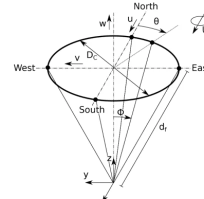
Figure 1.Lidar geometry definitions and coordinate system.

of the wind that are oriented in line with the mean wind di-rection (u) and vertical direction (w). This eliminates the av-eraging along the measurement circle.

The aim of the research presented here is to demonstrate whether one of the two modified data processing algorithms or their combination leads to improved turbulence measure-ments from standard VAD wind lidars. For each method, we present a numerical model and experimental results. We dis-cuss the effects of the two methods individually and com-bined.

This research has several practical applications. The reli-able elimination of cross-contamination and averaging along the measurement circle would lead to a reduction of the systematic error of wind lidar measurements that is depen-dent on the prevailing wind conditions and the measurement height. In particular, estimations of the timescale of turbu-lence could be made with higher certainty, which would sup-port future boundary layer research by means of profiling wind lidars. In addition, estimating the energy content of the wind components at specific wave numbers with higher cer-tainty could also help to better predict the operational wind loads of wind turbines and other structures.

2 Lidar theory

2.1 Coordinate system and preliminaries

Figure 1 shows the measurement circle of diameterDCof a VAD scanning lidar and how it is created by the laser beams that are deflected from the zenith by the half-cone open-ing angle φand rotate around the zenith with continuously changing azimuth angleθ. The beams are focused at a point at distancedffrom the lidar, which is located at the origin of a three-dimensional left-handed coordinate system. Five of the laser beams are depicted, four in the cardinal directions and one with an arbitrary azimuth angle. The mean wind di-rection2determined from 10 min intervals is zero when the wind blows from north to south. The wind vector

u= 

 u v w



 (1)

is composed of the wind components u, v andw that are aligned with the axes of the coordinate system when2=0◦. Reynolds decomposition is used for the description of the wind field so that

u=U+u0, (2)

whereu0 represents the wind speed fluctuations in all three directions andU is the mean wind velocity vector.

2.2 Taylor’s frozen turbulence hypothesis

The frozen turbulence hypothesis published by Taylor (1938) assumes that turbulence is advected by the mean wind ve-locityU into the mean wind direction2. During the trans-port process the turbulence remains unchanged, i.e., turbu-lence measured at one point in space gives information about the turbulence found further downwind some time later. That means for a velocity vector fielduwhenU is aligned with thex axis that

u(x, y, z, t )=u(x−Ut, y, z,0). (3) The hypothesis is widely used and it is known from exper-iments that the assumption of frozen turbulence is valid to a high degree for large eddies. For example, Schlipf et al. (2010) measured the inflow velocities of an operating wind turbine at different distances from the rotor plane in order to test the hypothesis of frozen turbulence. They found it to be valid for large-scale wind fluctuations with wave numbers

k >1.25×10−1m−1. Willis and Deardorff (1976) show that the hypothesis lacks validity when

σu/U>0.5. (4)

This implies that the validity of the hypothesis depends on the amount of turbulence and that a high degree of validity is expected when the velocity variance is low compared to the mean wind speed.

2.3 VAD measurement principle

Continuous-wave wind lidars continuously emit a focused in-frared laser beam into the air and detect the small portion of the radiation that is backscattered by particles along the beam path towards the beam’s origin. The velocity of the backscattering particles relative to the beam direction is then determined by analyzing the Doppler shift between the fre-quencies of outgoing and incoming radiation. It is assumed that the backscatterers are lightweight enough to move with the instantaneous wind speedu. The measured radial line-of-sight velocities vr are hence equal to the wind velocity projected onto the beam direction. In order to estimate the three-dimensional wind vectoru, a minimum of three inde-pendent line-of-sight measurements from different directions must be combined.

When VAD scanning is used, the beam is deflected by a wedge prism by a constant half-cone opening angle φ

from the zenith and rotated around the zenith with a steadily changing azimuth angleθ. Many radial velocitiesvrare ac-quired during one full rotation of the prism. For example in the case of the ZX 300 (previously ZephIR 300), N=49 Doppler spectra are calculated and used to determine the same number of radial velocities. All of them are used to reconstruct one wind vector by applying a least-squares fit to

vr= |Acos(θ−B)+C|, (5)

where the best fit parametersA,BandCrepresent the wind data according to

vhor=A/sin(φ)

2=B±180◦

vver=C/cos(φ). (6)

The sign of the radial velocity is usually unknown. We are thus faced with a directional ambiguity of±180◦, but this does not affect the turbulence analysis here. The wind data

vhor,2andvvercan be translated into wind vectorsueasily. The wind velocity estimations that result from this pro-cessing underlie several effects that distinguish them from one-point measurements. These effects can be divided into

– averaging

a. along the lines of sight

b. along the measurement circle and – cross-contamination

a. due to longitudinal separation b. due to lateral separation. 2.4 Averaging effects

2.4.1 Line-of-sight averaging

Table 1.Key specifications of the lidar used in the measurements.

Description Abbr. Value Unit

Measurement height h 78 [m] Half-cone angle φ 30.6 [◦] Cone diameter DC 92.3 [m] Focus distance df 90.6 [m] Prism rotation fS 1 [Hz] Measurements per cycle N 50 [1] Laser wave length λ 1550 [nm] Effec. aperture diam. a0 24 [mm] Mean wind speed Umean 19.5 [m s−1] 1. Resonance λres1 184.5 [m]

kres1 0.034 [m−1] 2. Resonance λres2 61.5 [m]

kres2 0.102 [m−1] No. of cycles to coverτ M 0–5 [1] Rayleigh length lR 7.03 [m] Full width at half maximum 2lR 14.07 [m]

volume that can be considered a point. Lidar measurements, in contrast, sense wind velocities along an extended stretch of the line of sight of the laser beam. In the case of continuous-wave lidars, the laser beam leaves the lidar optics with a di-ameter that corresponds to its effective aperture sizea0and is focused onto a focus point. The distance between the lidar optics and the focus point is the focal distance df. The sig-nal of the backscattered radiation originates from anywhere along the illuminated beam, according to a distribution func-tion that has its maximum at the focus point and is propor-tional to the intensity of the laser light along the beam (Son-nenschein and Horrigan, 1971).

A definite range gate, such as for pulsed lidars, is there-fore not applicable to continuous-wave lidars. Instead, the Rayleigh lengthlRis a measure of the distance between the focus point and the point at which the cross section of the beam has twice the area of the cross section at the focus point. According to Harris et al. (2006), it is given by

lR=

λdf2

π a02

, (7)

whereλis the laser wavelength anda0is the effective aper-ture diameter. The Rayleigh length is quadratically propor-tional to the focal distancedfthat increases linearly with the selected measurement height level. The degree of line-of-sight averaging is thus strongly dependent on the measure-ment height level and is higher for larger heights. The values oflR,a0anddffor the lidar used in our experiments are given in Table 1.

The intensity of backscattered radiation is a function of the distancesfrom the focus point along the beam. It is suf-ficiently well approximated by a Lorentzian function,

F (s)= lR/π s2_+l

R2

, (8)

wheresis the distance from the focus position (Mikkelsen, 2009).

All Doppler spectra that are retrieved during the radial velocity acquisition time are averaged, and the focus point sweeps over a considerable arc of the measurement circle during this time. This arc lengthlAis

lA=

DCπ

N , (9)

where N is the number of line-of-sight measurements vr taken during one rotation. In experimental data, the arc aver-aging effect is contained in the radial velocities. In the mod-els here, we account for this by averaging along the measure-ment circle.

The Doppler spectra of each line-of-sight measurement re-semble the probability density function of the radial wind ve-locities along the line of sight (Branlard et al., 2013). But by determining one single velocity value for each line-of-sight measurement, the turbulence information they contain is fil-tered out.

The additional temporal averaging along the lines of sight is very low, as one measurement takes only _N1 s. The effect of line-of-sight averaging is very strong for high wave num-bers but has some effect on long turbulent structures as well. The effect of line-of-sight averaging is considered in the nu-merical models and the discussion in this study. But none of the presented data processing methods can avoid the line-of-sight averaging effect.

2.4.2 Measurement circle averaging

As described in Sect. 2.3 lidars use all measurement data of at least one full rotation of the prism to reconstruct one wind vector. The resulting system of equations is overdetermined, and in order to find a solution a quadratic best fit is applied. The more line-of-sight velocities that are used to reconstruct a wind vector, the stronger the averaging and thereby the larger the loss of turbulent kinetic energy in the measurement data. The residual of the best fit is a measure of the degree of this form of averaging but is usually not used in the process-ing.

The diameterDCof the measurement circle is

DC=2htanφ, (10)

withh being the measurement height and φ the half-cone opening angle. The spatial separation between the points that one reconstructed wind vector is composed of thus linearly increases with measurement height. The larger the cone di-ameter, the stronger the circle averaging. Turbulence with a length scale below the diameter of the averaging circle is af-fected the most.

while it is probed, which might further increase the separa-tion of measurement points in the mean wind direcsepara-tion. The ZephIR 300 measures one full rotation in 1 s, and the distance the air moves within this time is usually small compared to

DC. The effect of temporal averaging is therefore often small compared to the spatial averaging. One example for the path of measurements that is averaged over is given in Fig. 4a. The circle diameter represents the spatial averaging, and the shift along-wind with the speed U represents the temporal averaging.

2.5 Cross-contamination

2.5.1 Cross-contamination due to longitudinal separation

Another cause for differences in the shape of turbulence spectra from one-point measurements and their counterparts from VAD scanning lidars is cross-contamination of differ-ent velocity compondiffer-ents. VAD scanning lidars combine mea-surements from spatially separated locations where differing velocities may prevail as if they were collected at one point. This leads to a redistribution of turbulent energy among the velocity components u, v andw. Lidar-derived spectra of one of the components can at certain wave numbers show lower energy values than the original wind spectrum of that component but may also show too high values due to a con-tribution from a different velocity component. To better un-derstand cross-contamination we divide the effect into two different types of separations. First we look into longitudinal separations, i.e., separation along the mean wind direction. Fluctuations at two points separated in line with the wind are highly correlated. If the assumption of frozen turbulence is correct, the coherence would be 1 for all separation lengths and all wave numbers. One example of cross-contamination of correlated fluctuations between two longitudinally sepa-rated points is visualized in Fig. 2. The chosen wavelength of the wind fluctuations equals twice the separation distance. This can be called the first resonance wavelength. The reso-nance wavelengths are given by

λres,n= 2DC

2n−1. (11)

The corresponding resonance wave numbers are

kres,n=

(2n−1)π DC

, (12)

where n=1, 2, 3. . . The resulting values for the first two resonance points are given in Table 1.

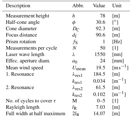
The two beam directions in line with and against the mean wind direction can be used to determineulidarandwlidarby using the formulas on the right-hand side of the figure. This example looks at these two lines of sight. Thevcomponent can be ignored because transverse fluctuations are not de-tected by the upstream and downstream beams. The example

Figure 2.Visualization of cross-contamination caused by longitu-dinal spacing of measurement points 1 and 2. The wavelength of u0andw0equals twice the separation distance of the focus points of the lidar (indicated by box with yellow symbol). The resulting measurement values of theucomponent are contaminated by fluc-tuations in thewdirection and vice versa.

demonstrates a case with isotropic turbulence, i.e., arbitrary but identical amplitudes for fluctuations in all orientations. Averaging along the lines of sight is ignored here for sim-plicity. The first column of graphs in the figure isolates the

ufluctuationsu0and shows the resulting lidar-measured sig-nal for the two radial velocities in the upwind and downwind directions, i.e.,vr1andvr2. When these two signals are bined in the usual way, the reconstructed wind speed com-ponentsu0_lidarandw_lidar0 differ strongly from the real inflow conditionsu0andw0. The lidar is blind to wind speed fluctua-tions in theudirection and instead attributes the fluctuations to some extent to the estimation ofw_lidar0 . The same is done forw0in the second column, and the resulting effect is the reverse. The vertical fluctuationsw0are interpreted solely as amplified fluctuations ofu0_lidar.

The last column combines the two previous cases and shows the resulting distribution of amplitudes that depends on the half-cone opening angleφ. Whenφ <45◦the lidar is more sensitive to vertical variations than to horizontal ones, and the contamination ofu0caused byw0is more severe than vice versa.

In a more realistic situation, turbulence is non-isotropic and the amplitude ofw0at this first resonance wave number is often considerably lower than the amplitude ofu0, which leads to a different distribution of contamination, which can be estimated as follows. We use Eqs. (31) and (33) to define the lidar-derived variance in theudirection:

σ_u,lidar2 = *

1v −2 sinφ

2+

In general, the differences of the line-of-sight velocities aligned with the mean wind 1v contain contributions from wind fluctuations in the uandwdirections1vu and1vw, respectively. Here we look at the resonance case in which

1vu=0 and thus1v=1vw. We get

σ_u,lidar,res2 = *

1vw −2 sinφ

2+ =

*

2w0cosφ −2 sinφ

2+

=cot2φσ_w,res2 ≈2.86σ_w,res2 , (14) when φ=30.6◦ as for the lidar we used in this study. The subscript “res” indicates that the equation is only valid for inflow fluctuations at resonance, as in the example given be-fore.

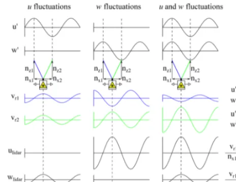
In Sect. 4 we develop a model to predict lidar-derived spectra. This model was used to create the plots shown in Fig. 3. Figure 3a shows the modeled spectra of the wind com-ponents, uwindandwwind, as solid black and red lines. The parameters of the underlying spectral tensor are given in Ta-ble 1. They were chosen to best represent the wind conditions found during the experiment presented in Sect. 6. The model was used to estimate theucomponent of the wind from two lidar beams that point in the upwind and downwind direc-tions. Also here, we did not include line-of-sight averaging to isolate the effect of cross-contamination. The principle of the setup is the same as explained for Fig. 2 but now we see results for all inflow wave numbers and use anisotropic tur-bulence. The resulting lidar-derived spectrumulidar,sumof the

ucomponent of the wind is the sum of the lidar’s interpreta-tion of the wind componentsulidar,uandulidar,w. We see that the lidar-estimated spectrum ofulidar,sumlies a bit below the target spectrum ofuwindfor most wave numbers but not at the first and second resonance points that are marked with grey dashed vertical lines. There it exceeds the target spectrum. The reason becomes apparent when we look at the compo-nentsulidar,u andulidar,w thatulidar,sum is composed of. We find that the lidar seesuwindnearly to its full extent for very low wave numbers but when we come close to the resonance pointsulidar,u drops to zero. The contribution of the vertical windulidar,wshows a mirrored behavior and is amplified ac-cording to Eq. (14) sinceφ <45◦.

2.5.2 Cross-contamination due to lateral separation When the lines of sight under consideration are not longitu-dinally but laterally separated, they do not face resonance but instead a second form of cross-contamination. The strength of the contamination depends then on the coherence of the turbulence for the given lateral separation. When the fluc-tuations at the two selected focus points are very coherent i.e., their correlation is close to unity, we can expect that the lidar-derived wind speed estimates are correct and no cross-contamination occurs. This can be observed at very low wave numbers at which a high degree of coherence is expected. The other extreme is found at the other end of the spectrum

Figure 3.Modeled cross-contamination effect inherent in(a)theu spectrum from two longitudinally separated points with1x=DC and (b) thev spectrum from two laterally separated points with 1y=DC. The solid lines are the spectra of the involved wind ponents. The dotted lines show the contribution of these wind com-ponents to the lidar spectra (circle markers). Averaging along the lines of sight is excluded.

at which small fluctuations measured at both focus points are uncorrelated. The lidar-derived spectrum is there a lin-ear combination of the variances of the involved components

vandwaccording to

σ_v,lidar2 = *

1v −2 sinφ

2+

= *

1vv −2 sinφ

2+ +

* 1vw −2 sinφ

2+

. (15)

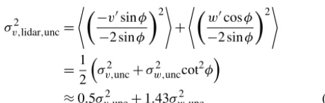
σ_v,lidar,unc2 of the lidar-derivedvvelocity is

σ_v,lidar,unc2 = *

_−v0_sinφ −2 sinφ

2+ +

*

_w0_cosφ −2 sinφ

2+

=1 2

σ_v,unc2 +σ_w,unc2 cot2φ

≈0.5σ_v,unc2 +1.43σ_w,unc2 (16) for the lidar with a half-cone opening angle of φ=30.6◦. These two situations and all cases in between are shown in Fig. 3b. The difference from the plots in Fig. 3a is that the two beams that point into and against thevdirection are used here to estimate thev-spectrumvlidar,sum. The target spectrum of thevcomponent of the windvwindis given as well as thew -spectrumwwindthat contaminates the signal. From thevlidar,v andvlidar,wcurves it can be seen that at very low wave num-bers hardly any contamination occurs but mainly because the

w-componentwwind itself contains a low energy density at low wave numbers. As it increases for higher wave numbers, the contamination also becomes more severe. In this exam-plewwinddominates the lidar spectrumvlidar,sumfor all wave numbers above approximatelyk1=1.4×10−2m−1. The re-sult is that the lidar overestimates the v variances for all wave numbers. Such an effect is also reported by Wyngaard (1968). Thus, it is essential for accurate turbulence measure-ments to minimize spatial separation.

VAD scanning along the whole measurement circle is more complex than using only two beams. Examining the two beams aligned with or perpendicular to the mean wind direction is not sufficient to fully understand the effect of cross-contamination. For circle scans, all three wind speed components are involved in contaminating all the beams that do not point in the four cardinal directions. We refer to the model presented in Sect. 4.1 and especially Eqs. (24), (25) and (26) of the spectral weighting functions therein to better understand which components influence another.

The lidar can also be configured to perform a so-called 3 s scan, in which one measurement cycle is built from data from three full rotations. This limits the cross-contamination but comes at the cost of much stronger averaging along the measurement circle, especially in strong wind cases, and a sampling rate that is 3 times slower. The ability to measure turbulence with this approach is so weak that it is not further investigated in this paper. Instead, the next chapter suggests two methods that can be used to reduce both averaging and cross-contamination.

3 Modified data processing 3.1 Squeezed measurement circles

In conventional VAD data processing, each measurement cy-cle consists of the radial velocities that are acquired during

one full rotation of the prism. The data used in the recon-struction of one wind vector thus originates from an air vol-ume with the shape of a cone with a diameter ofDCat the height of focus. This results in the abovementioned cross-contamination effects.

One way to eliminate the cross-contamination due to lon-gitudinal separation and mitigate the averaging along the measurement circle lies in making use of Taylor’s frozen tur-bulence hypothesis. As mentioned in Sect. 2.2, the hypoth-esis assumes that turbulent structures are transported by the mean wind motion without changing. This implies that all turbulent structures that enter the measurement cone at one time are identical after some timetwhen they leave the cone. The time it takes to cross the measurement circle can be esti-mated for all azimuth directionsθby

t (θ )=cosθDC

U , (17)

whereU is the mean wind velocity calculated from conven-tional VAD processing.

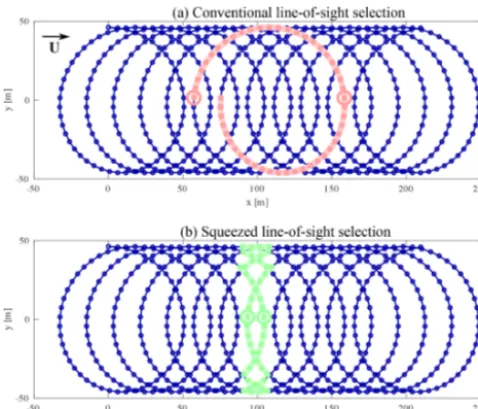
The basic idea here is to introduce a time lagτ=t into the data processing so that each air package that is involved in the reconstruction of one wind vector is scanned twice: once when it enters and again when it leaves the measure-ment cone. The composition of the measuremeasure-ment circles is shown in Fig. 4 from a coordinate system that is moving with the mean windU. In this exampleDC=92.3 m and

U=19.5 m s−1. With conventional VAD data processing, the measurement circle is made up of allNconsecutive mea-surements from one cycle (red segment). By contrast, the lower part of Fig. 4 illustrates the introduction of the time delayτ, in which line-of-sight measurements from a total of

M=6 different measurement cycles are combined to esti-mate one wind vector (green segments). In other words, with conventional data processing, a measurement cycle is com-posed of volumes that are widely spatially distributed. The new proposed method picks measurement data taken from what we term a squeezed measurement circle (SMC).

A restriction that comes with the idea of squeezing is that the circle sample ratefSmust be high enough to be able to select measurements that were acquired with a time differ-ence reasonably close toτ. That drastically limits the number of measurement heights that should be selected, especially in strong wind cases. For the measurements analyzed in this pa-per, the lidar scanned continuously at only one height level, which in general makes sense to measure turbulence effec-tively.

3.2 Two-beam method

Figure 4. Selection of line-of-sight measurements for the recon-struction of one wind vector for when (a, in red) conventional VAD processing and (b, in green) the method of squeezed measure-ment circles is applied. Within the red and green segmeasure-ments, small red and green rings indicate the particular beams selected for two-beam processing. In this example,U=19.5 m s−1, DC=92.3 m andfS=1 Hz.

it to determine the two beams that lie in the upstream and downstream directions. Within the red and green segments of Fig. 4, small red and green rings indicate these particular beams. These two beams can in a second processing step be used to estimate theuandwcomponents of the wind vectors for turbulence estimations. The resulting values are then not averaged along the measurement circle. This is comparable to the DBS method in cases in which the mean wind blows in line with two of the lines of sight. But an advantage of the two-beam method over the DBS strategy is that the relative angle between the mean wind and the two beams is kept con-stant in any prevailing wind direction. This is an advantage since beams pointing upwind and downwind are immune to contamination by the cross-wind componentv.

When the two-beam method is combined with the idea of squeezing, then measurements of theu andw components are taken at virtually one focus point following the flow. Only the line-of-sight averaging and some minor longitudinal sep-aration among the different locations along the two beams remain.

That is unfortunately not true when estimating thev com-ponent of turbulence. Instead, several problems occur. Intu-itively, one would choose a beam direction perpendicular to the mean wind direction in order to estimate thev compo-nent of the wind. But the radial velocities in this line-of-sight direction are often close to zero, and such estimates from continuous-wave lidars are usually not reliable (Mann et al., 2010; Dellwik et al., 2010). The transversev

compo-nent must therefore be estimated by either VAD processing or selecting a different third beam direction. In the latter case the results would then be influenced by contamination not only fromw but also from theucomponent. This lies out-side the scope of this study. Therefore novdata from mea-surements are processed with the two-beam method.

Like conventional VAD processing, the SMC method and two-beam method require a wind field that is statistically ho-mogeneous in the horizontal directions to yield correct re-sults.

4 Description of the model

The mathematics of deducing the lidar-measured spectrum from the second-order statistics of turbulence is very con-voluted. Therefore, we make the assumption that the mea-surements are performed much faster than it takes the air to move from one side of the scanning circle to the other; i.e., we assume that _f1

S τ. Effectively, the scanning circle is measured continuously. It is difficult to assess the magnitude of the error committed by the assumption of continuous mea-surements, but we assume it is negligible.

4.1 VAD and SMC

In order to model spectra obtained from conventionally VAD-processed lidar data, we closely follow the method of Sathe et al. (2011). They use the geometry of the lidar scan and its along-beam weighting function together with infor-mation on the spatial structure of surface-layer turbulence (Mann, 1994). The focus point of the lidar is at a distance

dfaway in the direction given by the unit vector

n(θ )=(−cosθsinφ,−sinθsinφ,cosφ) , (18) whereθis the azimuth angle andφis the half-cone opening angle. The line of sight or radial wind speed that the lidar is measuring is modeled as

vr(θ, x)= ∞ Z

−∞

ϕ(s)n(θ )·u((s+df)n(θ )+xe1)ds, (19)

whereϕ is the spatial weighing function of the continuous-wave lidar that we assume to be a Lorentzian function with the Rayleigh lengthlR.uis the three-dimensional velocity field suppressing the time argument since we are assuming Taylor’s hypothesis. The integration variablesis the distance along the beam from the focus point. The dot product assures that we obtain the line-of-sight velocity. We usex, the coor-dinate aligned with the mean wind vector, instead of time.e1 is the unit vector aligned withx.

i.e.,wis calculated from

A(x)= 1 2π

2π Z

0

vr(θ, x)dθ. (20)

In Sathe et al. (2011) variances are calculated for a conically scanning continuous-wave lidar and it is trivial to extend that to spectra. Spectra were in fact calculated in Sathe and Mann (2012) but only for a pulsed system. In Sathe et al. (2011) the variances for a conically scanning continuous-wave system, e.g., a ZephIR 300 (Smith et al., 2006; Kindler et al., 2007), were given by

D

w2Ecos2φ= Z

8ij(k)αi(k)α∗j(k)dk, (21) D

u2Esin2φ= Z

8ij(k)βi(k)βj∗(k)dk, (22) D

v2Esin2φ= Z

8ij(k)γi(k)γj∗(k)dk, (23) where∗means complex conjugation. The spectral weighting functionsα,β andγ are

αi(k)= 1 2π

2π Z

0

ni(θ )eidfk·n(θ )e−l|k·n(θ )|dθ, (24)

βi(k)= 1

π

2π Z

0

cosθ ni(θ )eidfk·n(θ )e−l|k·n(θ )|dθ, (25)

γi(k)= 1

π

2π Z

0

sinθ ni(θ )eidfk·n(θ )e−l|k·n(θ )|dθ. (26)

The spectra measured by the conically scanning lidar will be

cos2φF_wZ(k1)= ˆTf(k1) ∞ Z Z

−∞

8ij(k)αi(k)α∗j(k)dk2dk3 (27)

and likewise for theuandvcomponents. ˆ

Tf(k1)=sinc2

k1Lf 2

, (28)

where sincx=sinx

x is included in Eq. (28) to account for the finite time of circle scanning before a velocity estimate is ob-tained.Lfis the mean wind speed multiplied with this finite time (see Sathe et al., 2011, for details).

To apply the method of squeezing and model the spectra we obtain from SMC processing, we now substitute Eq. (19) with

evr(θ, x)= ∞ Z

−∞

ϕ(s)n(θ )·u((s+df)n(θ )+(x−dfn1(θ ))e1)ds .

(29) Following the exact same steps as in Sathe et al. (2011) but using Eq. (29) instead of Eq. (19) we arrive at Eqs. (21)– (23) but with the complex exponential in Eqs. (24)–(26) ex-changed with

eidf(k·n(θ )−k1n1(θ ))_{. (30)} 4.2 Two-beam method

Only the up- and downwind beams to determine theuandw

components of the wind vector could introduce less averag-ing than usaverag-ing the whole circle.

When the mean wind is blowing from the north, the unit vectors in the up- and downwind directions are callednuand

nd, respectively. Their unit vectors are

nu=(−sinφ,0,cosφ) (31)

and with the opposite sign on the first component fornd. Parallel to Eq. (19) the line-of-sight velocity measured by the upwind beam is assumed to be

vu(x)= ∞ Z

−∞

ϕ(s)nu·u(snu+dfnu+xe1)ds. (32)

Theucomponent estimated by the lidar is normally

ulidar=

1v

nu₁−nd₁, (33)

where

1v=vu(x)−vd(x)

= ∞ Z

−∞

ϕ(s)nu·u((s+df)nu+xe1)

−nd·u((s+df)nd+x)ds. (34) The correlation function of1vis

R1v(r)= h1v(x)1v(x+r)i

= ∞ Z Z

−∞

ϕ(s)ϕ(s0)×Dnu·u((s+df)nu+xe1)

−nd·u((s+df)nd+xe1) ×nu·u((s0+df)nu+(x+r)e1)

−nd·u((s0+df)nd+(x+r)e1) E

field,Rij(r)≡ui(x)uj(x+r), one obtains

R1v(r)= ∞ Z Z

−∞

ϕ(s)ϕ(s0)× (36)

n

nu_inu_jRij((−s+s0)nu+re1)

+nd_ind_jRij((−s+s0)nd+re1)

−nu_ind_jRij(s0nd−snu+df(nd−nu)+re1)

−nd_inu_jRij(s0nu−snd+df(nu−nd)+re1) o

dsds0.

Now we use the relation between the velocity covariance ten-sor and the spectral velocity tenten-sor

Rij(r)= Z

8ij(k)exp(ik·r)dk, (37)

where R

dk≡R R R_−∞∞ dk1dk2dk3, to express the auto-covariance function as

R1v(r)= ∞ Z Z

−∞

ϕ(s)ϕ(s0)

× n

nu_inu_j Z

8ij(k)

exp ik·((−s+s0)nu+re1

dk +nd_ind_j

Z 8ij(k)

expik·((−s+s0)nd+re1

dk −nu_ind_j

Z 8ij(k)

expik·(s0nd−snu+df(nd−nu)+re1

dk −nd_inu_j

Z

8ij(k)exp

ik·(s0nu−snd+df(nu−nd)

+re1

dkodsds0. (38)

By interchanging the order of integration of k and thes’s we can cast the expression in terms of the Fourier trans-form of ϕ, which in the case of a Lorentzian function is

ˆ

ϕ(k)=exp(−lR|k|). Thereafter, we Fourier transform R1v with respect tor to obtain the spectrumF1v(k1). After that process the first term in Eq. (38) becomes

nu_inu_j Z

8ij(k)ϕ(kˆ ·nu)ϕ(kˆ ·nu)dk2dk3,

and upon rearrangement we finally obtain

F1v,n(k1)= Z

8ij(k)

nu_inu_jϕ(kˆ ·nu) 2

+nd_ind_j ϕ(kˆ ·n

d₎ 2

−2nu_ind_jϕ(kˆ ·nu)ϕ(kˆ ·nd) (39) ×cosdfk·(nd−nu)

dk2dk3.

The derivation of the spectrum obtained from squeezed pro-cessing is parallel to the normal spectrum. The only differ-ence lies in the definition of1v. Now we define it as

1vs(x)=vu(x−nu1df)−vd(x−nd1df). (40) Using the exact same steps that led to Eq. (39), we see that the cosine term in that equation has to be substituted with 1 and we get

F1v,s(k1)= Z

8ij(k)

nu_inu_jϕ(kˆ ·nu) 2

+nd_ind_j ϕ(kˆ ·n

d₎ 2

−2nu_ind_jϕ(kˆ ·nu)ϕ(kˆ ·nd)

dk2dk3. (41) To obtain the spectrum ofu,F1v,(s)simply has to be divided by(nu₁−nd₁)2according to Eq. (33).

When obtaining the spectrum ofv, we simply exchange the unit vectors of the up- and downwind beamsnuandndin all equations by the values of the west- and eastbound beams

nwandne. In order to obtain the spectrum ofw,1vdefined in Eq. (34) has to be replaced by the sum of both radial ve-locitiesvu(x)+vd(x), andF1v,(s)must eventually be divided by(nu₃+nd₃)2.

To compare the different methods to calculate spectra from a lidar, Eqs. (39) and (41) have to be evaluated with a model for the spectral tensor. We chose the spectral tensor from Mann (1994) and select the model parameters so that the model spectra resemble the spectra from available sonic mea-surements. The selected parameters areL=65 m,0=4 and

α23 =0.023 m43_s−2_{. The unfilteredutarget model spectrum} that we will later compare the model results against is given by

Fu(k1)= Z

811(k)dk2dk3 (42)

5 Description of the measurements 5.1 Test site and instrumentation

The test data were collected at the Danish National Test Cen-ter for Large Wind Turbines at Høvsøre. The test site is lo-cated in West Jutland, Denmark, 1.7 km east of the North Sea. Apart from the dunes along the coastline, the terrain is nearly flat. The Høvsøre meteorological mast is located to the south of a row of five wind turbines. The reference data were acquired with a Metek USA-1 sonic anemometer that is mounted at 80.5 m in height above the ground. It is at-tached to a 4.3 m long boom pointing north. Mast effects can be observed when the wind is blowing from the south. Tur-bine wake effects influence the measurement signal when the wind blows from the north. For the data set in this study, the inflow is undisturbed. A detailed description of the test site is given in Peña et al. (2016).

Collocated with the meteorological mast, the lidar mea-surements were taken by a Qinetiq lidar that was configured to continuously scan at 78 m above the ground. The lidar is comparable to the current ZX 300 (previously ZephIR 300) but the effective aperture size is slightly lower, which results in a longer Rayleigh length and thus greater line-of-sight av-eraging. The lidar was equipped with an opto-acoustic mod-ulator that makes it possible to detect the direction of the radial velocities. Line-of-sight velocities calculated from the centroid of the Doppler spectra are used in the data process-ing. The precision of these lidar measurements is not ex-actly known but is in general better than 1 % (Pedersen et al., 2012).

Measurement data of 32 subsequent 10 min intervals are used. The data were acquired on 20 November 2008 between 10:30 and 15:50 local time. The mean wind velocity mea-sured by the sonic anemometer during this period varied from 14.2 to 22.6 m s−1with an average of 19.5 m s−1and a stan-dard deviation of 2.0 m s−1. The turbulence intensity varied from 4.7 % to 14.0 %, with a mean of 8.8 % and standard deviation of 2.0 %. The wind blew from the northwest and the atmospheric stability was neutral. Table 1 summarizes the most important information about the experimental setup. 5.2 Data processing

The time series of all 10 min intervals derived from all pro-cessing methods are used to compute turbulence spectra. The measurement rate for the lidar is 1 Hz. Although it would have been possible in the two-beam processing to calculate measurement values with a rate of 2 Hz by using every newly retrieved radial velocity together with its predecessor, it was decided to use only independent measurements acquired ev-ery full second. The sonic anemometer measures with a rate of 20 Hz. These high-frequency data are down-sampled by the use of the MATLAB function “resample” to a frequency of 1 Hz. The function includes a low-pass filter to avoid

anti-aliasing. The data rate is thus for all methods 1 Hz. The an-alyzed frequency range from ₆₀₀1 to 1₂Hz equals the wave number range from roughly 5.4×10−4to 1.6×10−1m−1. The spectra are then averaged for all intervals and the results are then binned into 30 logarithmically spaced wave number intervals spread across the wave number axis to avoid high density of values and maintain readability towards higher wave numbers.

The effects of de-trending (Hansen and Larsen, 2005) and spike removal (Hojstrup, 1993) on the spectra were both neg-ligible for this data set, so neither was applied here.

6 Discussion of the results 6.1 uspectra

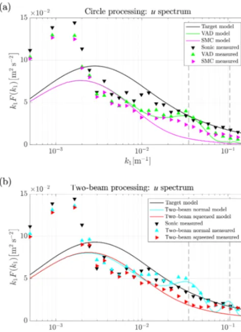
Figure 5 shows the spectra of theufluctuations for all pro-cessing methods from measurement data (triangle markers) and the corresponding model predictions (solid lines). We will first discuss the results from processing the whole mea-surement circle shown in Fig. 5a, followed by the discussion of the results of the two-beam method, shown in Fig. 5b. 6.1.1 Circle processing

To begin with, the model predictions of conventional VAD processing and the new SMC method are compared against each other and with regard to the trueutarget model spec-trum acquired from the spectral tensor according to Eq. (42). The model prediction of the conventionally processed VAD lidar data shows some attenuation of the spectral energy even for very low wave numbers. This can be partly explained by the infinitely long tails of the line-of-sight averaging func-tion given in Eq. (8). That means that even very large eddies are slightly weakened by the underlying Lorentzian func-tion. Averaging along the measurement circle might also have some small additional impact on large-scale turbulence. Both averaging effects become more and more severe for in-creasing wave numbers until the measured spectral energy reaches values close to zero at roughlyk1=10−1m−1 and above. The tendency of increasing attenuation with regard to the target spectrum is interrupted around the first resonance frequency that is indicated by a vertical grey dashed line at

k1=3.4×10−2m−1. Here the energy density increases and reaches coincidentally roughly the value of the target spec-trum. This behavior is as expected an effect of the cross-contamination with energy from both thewspectrum and to a small extent also fromv. A resonance effect at the second resonance frequency is hardly pronounced since the energy is nearly fully consumed by the line-of-sight averaging.

con-Figure 5.Modeled (solid lines) and measured (triangle markers)u spectra from data processing for which(a)all radial measurements are used and(b)only two beams are used. Colors correspond to the processing method. The grey vertical dashed lines represent the first and second resonance wave numbers.

tained in the uSMC signal. The signal is still contaminated by contributions from other components because the lateral separation cannot be reduced by squeezing. But the averag-ing along the measurement circle is so strong that for exam-ple for wave numbers above aroundk1=10−2m−1less than half of the energy of the target spectrum is expected to be detected by the lidar.

First, when the model is compared with the measurement data, the chosen spectral tensor does not fit the actual wind conditions in the wave number range belowk1=10−2m−1. The extra energy at low wave numbers compared to the spec-tral tensor model for this site has been observed before and is related to the inhomogeneous landscape at Høvsøre with its sea-to-land transition in the main wind direction (Sathe et al., 2015) and mesoscale effects that overlay the expected spec-tral gap (Larsén et al., 2016). Luckily, this does not severely impede the analysis since the most interesting effects are ex-pected at higher wave numbers and tendencies can still be determined from the relative distances between the markers and lines without matching the absolute values. Next, the

comparison of data from sonic measurements and VAD as well as SMC-processed lidar data shows in the very low wave number range atk1<3×10−3m−1that VAD processing and SMC processing produce similar results with a slight ten-dency towards lower energy densities in the SMC-measured spectrum that is not found in the model computations. A pos-sible explanation is that the fluctuations of theu and espe-cially thew component in the real wind field are not per-fectly correlated, i.e., the frozen turbulence hypothesis that the model assumes is slightly violated. The result is a small contribution ofwwindtoulidarthat appears to a greater extent in the VAD-processed spectrum. The reason for the differ-ence is that the correlation is closer to unity in the case of SMC processing.

Apart from some exceptions (e.g., atk1=3×10−3m−1), a relatively increasing averaging effect towards higher wave numbers is found for the lowest wave numbers as expected. In the wave number rangek1=10−2 to 6×10−2m−1 the sonic spectrum and the VAD spectrum follow the corre-sponding modeled spectra nicely through the first resonance point. That shows that the cross-contamination caused by longitudinal separation is present in the measurements and is properly modeled.

The spectrum derived from SMC-processed data shows a clear tendency towards its modeled spectrum but does not completely reach it. It does not show the resonance effect seen for VAD processing, but the overall energy level is higher than predicted fork1>10−2m−1. It is not possible to determine what causes this deviation. One possible reason is that the model assumes a perfect delay of the measurement timing. In reality this is not possible due to only discrete ac-quisition times being available. Also the air packages are in reality not always advected with the exact mean wind speed and direction. Both imperfections justify that the behavior of real SMC processing lies in between the modeled SMC and VAD processing.

Fork1>7×10−2m−1VAD- and SMC-processed data are nearly identical. As shown in Schlipf et al. (2010), the as-sumption of frozen turbulence is not valid for high wave numbers. In this region, fluctuations separated by the dis-tances between the relevant focus points are uncorrelated and the squeezing has no effect. The lack of coherence also ex-plains that the values are higher than predicted because theu

spectrum is highly contaminated bywandvfluctuations. 6.1.2 Two-beam processing

The plotted model spectrum for the conventional two-beam processing method shows a significantly lower averaging ef-fect compared to whole circle processing methods at all wave numbers except in the very low wave number region, where the methods are expected to perform similarly well.

when circle processing was applied. The normal two-beam processing in the model is prone to cross-contamination at both resonance points (vertical dashed lines). This situation is explained in detail in Sect. 2.5. In contrast, the method of squeezing applied to the two-beam processing shows as ex-pected no cross-contamination in the model calculations.

Overall, spectra calculated from the two-beam processed measurement data show good agreement to the model. It is important to keep in mind that, due to the poor fit of the measured spectra of the horizontal wind components and the modeled spectra at low wave numbers, we can com-pare the relations between the different methods but not ab-solute values. At low wave numbers, the measured spec-tra are on average closer to the target spectrum than in the case of circle processing. The slightly lower energy content of squeezed measurements that we observed and explained for circle processing is found here as well. Also, when it comes to deviations from the modeled behavior, like for ex-ample the higher energy density at some wave numbers (e.g.,

k1=3×10−3m−1), we find similar tendencies as in circle processing, and the reason is likewise unclear.

The strong cross-contamination at the first resonance fre-quency is clearly represented in the normal two-beam pro-cessing and can be completely avoided by squeezing the two focus points to virtually one point. It is worth mentioning that the squeezing procedure works more like expected when ap-plied to the two-beam method than when apap-plied to the circle processing. This can be explained by the error caused by not having continuous but only discrete delaying times τ avail-able. The relative impact of this error is lower in the case of the two-beam method because then the maximum separation distance DCmust be compensated for. In circle processing mode, the shorter separations for which the relative error is larger also contribute to the result.

Atk1>7×10−2m−1the two processing methods result in nearly identical values again, and we assume the lack of coherence of short eddies to also be the cause here.

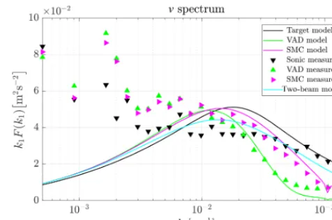
6.2 vspectra

Figure 6 shows the spectra of thevfluctuations for all avail-able data processing methods from both measurement data (triangle markers) and the corresponding model predictions (solid lines). Also here, we first discuss the results from processing the whole measurement circle shown in Fig. 6a, followed by the discussion of the results of the two-beam method shown in Fig. 6b.

6.2.1 Circle processing

The modeled spectra of conventionally VAD-processed li-dar measurements predict energy densities that slightly ex-ceed the target spectrum for very long fluctuations withk1< 1.3×10−2m−1. This behavior can be explained by uncorre-latedwfluctuations between the eastern and western sides of

Figure 6.Modeled (solid lines) and measured (triangle markers) vspectra from all data processing methods. Colors correspond to processing method.

the measurement circle that contaminate thev signal. This contamination is slightly stronger than averaging that is very weak at low wave numbers.

By contrast, fluctuations shorter than approximatelyk1= 1.3×10−2m−1appear dampened in the spectrum, and fluc-tuations with higher wave numbersk1>10−1m−1 are not even present in thev spectrum due to the strong averaging. Unlike theuspectrum, thev spectrum does not have char-acteristic behavior around the first resonance wave number. This is not surprising because the lines of sight that are the most important for the detection ofvfluctuations lie, accord-ing to Eq. (26), orthogonal to the mean wind direction in which turbulence is advected. Thus, no resonance occurs.

measure-ment circle when SMC is applied. As a result, the spectrum of SMC shows higher energy densities for all wave numbers at which uncorrelated fluctuations dominate.

Now we compare the measurements with the model. Un-fortunately, similar to theufluctuations, the target spectrum does not represent the sonic measured values properly, es-pecially for low wave numbers. We will therefore concen-trate on the tendencies and proportions between the spectra from different methods. While the model predicts the behav-ior at the lowest wave numbers more or less satisfactorily, we are faced with two outliers atk1=1.65×10−3m−1and

k1=2×10−3m−1for which both the VAD and SMC pro-cessing lead to excessive energy estimations. The reason is unclear and not further investigated. At all other wave num-bers, the agreement of model and measurements is very satis-factory. In particular, the differences between the two meth-ods are found in the measurements, as predicted. The good agreement between model spectra and measurement spectra at wave numbers above approximately k1=2×10−2m−1 might be surprising with regard to the poor agreement of sonic measurements and target spectrum. The reason is that the shape of the lidarvspectra is mainly determined by the cross-contamination from the w component, which, as we describe in Sect. 6.3, agrees better with its model representa-tion.

The identity of VAD- and SMC-derived measurement spectra that we saw forufluctuations fork1>7×10−2m−1 is found here atk1>10−1m−1. The reason is obvious when we look at the relevant longitudinal separation distances. They are much shorter when processingvfluctuations thanu

fluctuations, and the assumption of frozen turbulence is more valid for short separation distances. Therefore squeezing can maintain its effect into a somewhat higher wave number re-gion.

6.2.2 Two-beam processing

When the two-beam method is applied, i.e., using only the east and west beams to derive thevcomponent of the wind vector, the method of squeezing has no effect. In comparison with the whole circle processing, the two-beam method is characterized by lower energy estimates at low wave num-bers and higher energy estimates at higher wave numnum-bers (see Fig. 6). One reason for the first is assumed to be the lower coherence ofv fluctuations separated by the full dis-tance DC. That implies that two-beam processing gets a somewhat lower contribution ofvwindtovlidar. A second rea-son is that there is not cross-contamination fromuonv oc-curring for the two-beam processing. The higher energy con-tent at high wave numbers results from the absence of aver-aging along the measurement circle.

The model cannot be compared with measurements be-cause the line-of-sight velocities of the east and west beams were erroneous. The absolute values we measured are unreal-istically biased towards nonzero values. This effect has been

Figure 7.Modeled (solid lines) and measured (triangle markers)w spectra from data processing for which(a)all radial measurements are used and(b) only two beams are used. Colors correspond to processing method. The grey vertical dashed lines represent the first and second resonance wave numbers.

previously reported (Mann et al., 2010; Dellwik et al., 2010). We included the model behavior of two-beam processing for the sake of completeness and to show that the availability of reliable measurement data for the east and west beams would be of hardly any use.

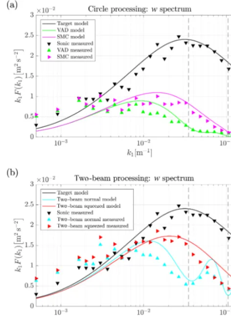
6.3 wspectra

Figure 7 shows the spectra of thewfluctuations for all pro-cessing methods from both measurement data and the cor-responding model predictions. Again, we discuss the results from processing the whole measurement circle first and then the results of the two-beam method.

6.3.1 Circle processing

some attenuation of the spectral energy even for very low wave numbers. The reason is mainly the infinitely long tails of the line-of-sight averaging function and to a lesser extent the averaging along the measurement circle. Both averaging effects become quickly stronger for increasing wave num-bers. The spectrum from VAD processed data is expected to drop at the first resonance point marked with a grey dashed vertical line in Fig. 7. This drop is minor due to the over-all low energy level present in the spectrum. The spectrum reaches a value near its final minimum with variance val-ues close to zero already at around k1=5×10−2m−1just after crossing the first resonance point. wfluctuations with higher wave numbers are not detectable with conventional VAD processing. According to the model, the SMC process-ing improves the situation slightly by removprocess-ing the longitu-dinal separation that makes lidar blind towfluctuations at the resonance points with VAD processing. Squeezing the mea-surements also helps improve the meamea-surements well above and below the resonance wave number. But still, due to the remaining averaging effects, only a minor fraction of the en-ergy in the vertical wind can be detected with both methods at wave numbers above roughlyk1=10−2m−1.

The fit between target spectrum and measurement data in the low wave number region is good for thew component. This was not the case for theuandvcomponents. The results of Larsén et al. (2016) show that the spectra for vertical fluc-tuations are not prone to contributions from the mesoscale spectrum. The measurement data overall support these model predictions and show that the process of squeezing functions well over the entire frequency range in this study. In detail, we only find some mismatch for very low wave numbers at which k1<10−3m−1. The measured spectra lie above the target spectrum here although we expected some attenuation. The discrepancy is caused by the realu-wind spectrum being much higher than the underlying target spectrum; see Fig. 5. We already found that large-scaleufluctuations are also not perfectly correlated and thus contaminate the measured li-dar spectra, which is not considered in the model. At higher wave numbers we find reasonable forecasting of measuredw

spectra by the model.

6.3.2 Two-beam processing

The modeled two-beam spectra in Fig. 7b lie considerably closer to the target wspectrum for all wave numbers. That can be explained by the absence of circle averaging. The strong influence of resonance visible at the two first reso-nance wave numbers underlines the importance of squeezing when striving for more realistic spectra from lidar measure-ments.

At low wave numbers withk1<10−2m−1 the measured spectra contain higher energy densities than modeled spec-tra. A similar but less pronounced effect was found in circle processing only at the lowest wave numbers. The explanation we gave there must therefore be supplemented by mentioning

that the assumed decorrelation is stronger for the maximal separations that are involved in the two-beam method. The further comparison of spectra from experiment and model shows that the process of squeezing also leads to the ex-pected effect in the case of using only two beams to deter-mine thewcomponent of the wind vector. As in the case of

ufluctuations, this statement must be limited to wave num-bersk1<7×10−2m−1.

6.4 Extended discussion

The results discussed here are extracted from a single data set that covers one measurement height and a narrow band of mean wind speeds, turbulence conditions and inflow di-rections at a single location. The reason for working with such a limited data set lies in the fact that very few data are available where a commercial VAD scanning wind lidar, col-located to a meteorological mast, is scanning continuously at one height level, while saving at least the line-of-sight veloci-ties. Currently, the only option to save line-of-sight velocities acquired by a ZephIR 300 is to stream the data manually to a connected PC. The situation is further complicated by the fact that in the normal “profiling mode” the lidar focuses to a reference height of 38 m periodically for filtering purposes. Therefore, the only known way to focus at one particular al-titude continuously is to switch the unit to “turbine mode”. In this way, we acquired some data for the investigation, but their overall quality was lower than the historic data that we eventually selected as the best available data.

mainly determined by the degree of anisotropy and the tur-bulence length scale. Atmospheric stability conditions other than neutral would not change the way the lidar measures. But a modified spectral tensor model like the one presented in Chougule et al. (2017) could be used to better compare model values with experimental results.

7 Conclusions

This paper presents two advanced data processing meth-ods for improving turbulence spectrum estimations with VAD scanning wind lidars, with an aim to reduce cross-contamination and averaging effects. The models of these approaches, developed in Sect. 4, are supported by the com-parison with experimental data. Discrepancies can be ex-plained for the most part by the limitations of the frozen tur-bulence hypothesis that underlies the model calculations yet has slightly reduced validity in real measurements. The fact that the spectra in the experiment do not agree very well with the spectral tensor model is also a cause of differences.

We found that the method of squeezing eliminates the res-onance effect caused by the longitudinal separation of com-bined measurement points successfully. It also considerably reduces the averaging along the measurement circle.

The method of using only two beams for the estimation of the uandw components of the wind vector eliminates the averaging along the measurement circle completely. When it is combined with the method of squeezing, the measure-ments deviate from the sonic measuremeasure-ments mainly due to line-of-sight averaging. This combination of both methods substantially improves the measurability of thewspectrum, which is hardly measurable with current VAD processing.

Accurate measurements of the v spectrum remain dif-ficult, even with the approaches described here. The two-beam method is not applicable to current continuous-wave lidars, which in most cases are homodyne. Whether the use of squeezed measurement circles always leads to systemat-ically better results is unclear because the resulting spectra are dominated by contamination fromwfluctuations of the wind.

In conventionally processed lidar data, cross-contamination compensates for averaging effects, meaning that in general total variance might be close to target values but for the wrong reasons. For systematically better turbulence measurements from VAD scanning lidars, the findings presented here should be included in raw data processing. Both approaches presented here can be applied to any existing VAD scanning continuous-wave profiling lidar unit.

Code and data availability. Inquiries about and requests for access to data and source codes used for the analysis in this study should be directed to the authors.

Competing interests. The authors declare that they have no conflict of interest.

Acknowledgements. This research project was supported by Energy and Sensor Systems (ENERSENSE) at the Norwegian University of Science and Technology.

Review statement. This paper was edited by Marcos Portabella and reviewed by two anonymous referees.

References

Bardal, L. M. and Sætran, L. R.: Spatial correlation of atmo-spheric wind at scales relevant for large scale wind turbines, J. Phys. Conf. Ser., 753, 32–33, https://doi.org/10.1088/1742-6596/753/3/032033, 2016.

Branlard, E., Pedersen, A. T., Mann, J., Angelou, N., Fis-cher, A., Mikkelsen, T., Harris, M., Slinger, C., and Montes, B. F.: Retrieving wind statistics from average spectrum of continuous-wave lidar, Atmos. Meas. Tech., 6, 1673–1683, https://doi.org/10.5194/amt-6-1673-2013, 2013.

Browning, K. A. and Wexler, R.: The Determination of Kine-matic Properties of a Wind Field Using Doppler Radar, J. Appl. Meteorol.Clim., 7, 105–113, https://doi.org/10.1175/1520-0450(1968)007<0105:TDOKPO>2.0.CO;2, 1968.

Canadillas, B., Bégué, A., and Neumann, T.: Comparison of turbu-lence spectra derived from LiDAR and sonic measurements at the offshore platform FINO1, 10th German Wind Energy Con-ference (DEWEK 2010), 17–18 November 2010, Bremen, Ger-many, 2010.

Chougule, A., Mann, J., Kelly, M., and Larsen, G.: Modeling Atmo-spheric Turbulence via Rapid Distortion Theory: Spectral Ten-sor of Velocity and Buoyancy, J. Atmos. Sci., 74, 949–974, https://doi.org/10.1175/JAS-D-16-0215.1, 2017.

Dellwik, E., Mann, J., and Bingöl, F.: Flow tilt angles near for-est edges – Part 2: Lidar anemometry, Biogeosciences, 7, 1759– 1768, https://doi.org/10.5194/bg-7-1759-2010, 2010.

Eberhard, W. L., Cupp, R. E., and Healy, K. R.: Doppler Lidar Mea-surement of Profiles of Turbulence and Momentum Flux, J. At-mos. Ocean. Technol., 6, 809–819, https://doi.org/10.1175/1520-0426(1989)006<0809:DLMOPO>2.0.CO;2, 1989.

Hansen, K. S. and Larsen, G. C.: Characterising Turbulence Inten-sity for Fatigue Load Analysis of Wind Turbines, Wind Eng., 29, 319–329, https://doi.org/10.1260/030952405774857897, 2005. Harris, M., Hand, M., and Wright, A.: Lidar for Turbine Control,

Tech. Rep. NREL/TP-500-39154, National Renewable Energy Laboratory, Golden, Colorado, USA, 2006.

Hojstrup, J.: A statistical data screening procedure, Meas. Sci. Tech-nol., 4, 153–157, 1993.

Kim, D., Kim, T., Oh, G., Huh, J., and Ko, K.: A com-parison of ground-based LiDAR and met mast wind mea-surements for wind resource assessment over various ter-rain conditions, J. Wind Eng. Ind. Aerodyn., 158, 109–121, https://doi.org/10.1016/j.jweia.2016.09.011, 2016.

Kindler, D., Oldroyd, A., Macaskill, A., and Finch, D.: An eight month test campaign of the Qinetiq ZephIR system: Preliminary

results, Meteorol. Z., 16, 479–489, https://doi.org/10.1127/0941-2948/2007/0226, 2007.

Larsén, X. G., Larsen, S. E., and Petersen, E. L.: Full-Scale Spec-trum of Boundary-Layer Winds, Bound.-Lay. Meteorol., 159, 349–371, https://doi.org/10.1007/s10546-016-0129-x, 2016. Mann, J.: The spatial structure of neutral atmospheric

surface-layer turbulence, J. Fluid Mech., 273, 141–168, https://doi.org/10.1017/S0022112094001886, 1994.

Mann, J.: Wind Field Simulation, Probab. Eng. Mech., 13, 269–282, https://doi.org/10.1016/S0266-8920(97)00036-2, 1998. Mann, J., Peña, A., Bingöl, F., Wagner, R., and Courtney,

M. S.: Lidar scanning of momentum flux in and above the surface layer, J. Atmos. Ocean. Tech., 27, 959–976, https://doi.org/10.1175/2010JTECHA1389.1, 2010.

Medley, J., Wylie, S., Slinger, C., Harris, M., des Roziers, E. B., Pitter, M., and Mangat, M.: Classification of ZephIR 300 Lidar at the UK Remote Sensor Test Site, EWEA Resource Assessment 2015, Helsinki, Finland, 2015.

Mikkelsen, T. K.: On mean wind and turbulence profile measure-ments from ground-based wind lidars: limitations in time and space resolution with continuous wave and pulsed lidar systems, European Wind Energy Conference and Exhibition 2009, 16–19 March 2009, Marseille, France, 6, 4123–4132, 2009.

Newman, J. F., Klein, P. M., Wharton, S., Sathe, A., Bonin, T. A., Chilson, P. B., and Muschinski, A.: Evaluation of three lidar scanning strategies for turbulence measurements, Atmos. Meas. Tech., 9, 1993–2013, https://doi.org/10.5194/amt-9-1993-2016, 2016.

Pedersen, A. T., Montes, B. F., Pedersen, J. E., Harris, M., and Mikkelsen, T.: Demonstration of short- range wind lidar in a high-performance wind tunnel, in: Poster presented at EWEA 2012 – European Wind Energy Conference & Exhibition, 16–19 March 2012, Copenhagen, Denmark, 2012.

Peña, A., Hasager, C. B., Gryning, S.-E., Courtney, M., Antoniou, I., and Mikkelsen, T.: Offshore Wind Profiling Using Light De-tection and Ranging Measurements, Wind Energy, 12, 105–124, https://doi.org/10.1002/we.283, 2009.

Peña, A., Floors, R., Sathe, A., Gryning, S.-E., Wagner, R., Court-ney, M. S., Larsen, X. G., Hahmann, A. N., and Hasager, C. B.: Ten Years of Boundary-Layer and Wind-Power Meteo-rology at Høvsøre, Denmark, Bound.-Lay. Meteorol., 158, 1–26, https://doi.org/10.1007/s10546-015-0079-8, 2016.

Sathe, A. and Mann, J.: Measurement of turbulence spectra us-ing scannus-ing pulsed wind lidars, J. Geophys. Res.-Atmos., 117, D01201, https://doi.org/10.1029/2011JD016786, 2012. Sathe, A. and Mann, J.: A review of turbulence measurements using

ground-based wind lidars, Atmos. Meas. Tech., 6, 3147–3167, https://doi.org/10.5194/amt-6-3147-2013, 2013.

Sathe, A., Mann, J., Gottschall, J., and Courtney, M. S.: Can wind lidars measure turbulence?, J. Atmos. Ocean. Tech., 28, 853–868, https://doi.org/10.1175/JTECH-D-10-05004.1, 2011.

Sathe, A., Mann, J., Vasiljevic, N., and Lea, G.: A six-beam method to measure turbulence statistics using ground-based wind lidars, Atmos. Meas. Tech., 8, 729–740, https://doi.org/10.5194/amt-8-729-2015, 2015.

applica-tions with a scanning LIDAR system, ISARS 2010, 28–30 June 2010, Paris, https://doi.org/10.18419/opus-3915, 2010.

Smith, D. A., Harris, M., Coffey, A. S., Mikkelsen, T., Jørgensen, H. E., Mann, J., and Danielian, R.: Wind lidar evaluation at the Danish wind test site Høvsøre, Wind Energy, 9, 87–93, https://doi.org/10.1002/we.193, 2006.

Sonnenschein, C. M. and Horrigan, F. A.: Signal-to-Noise Relationships for Coaxial Systems that Heterodyne Backscatter from the Atmosphere, Appl. Optics, 10, 1600, https://doi.org/10.1364/AO.10.001600, 1971.

Taylor, G. I.: The Spectrum of Turbulence, P. Roy. Soc. A, 164, 476–490, https://doi.org/10.1098/rspa.1938.0032, 1938.

Wagner, R., Mikkelsen, T., and Courtney, M.: Investigation of turbu-lence measurements with a continuous wave, conically scanning LiDAR, Risø-R-1682(EN), DTU, Risø, Denmark, 2009. Willis, G. E. and Deardorff, J.: On the use of Taylor’s translation

hypothesis for diffusion in the mixed layer, Q. J. Roy. Meteorol. Soc., 102, 817–822, https://doi.org/10.1002/qj.49710243411, 1976.