BIOGEOGRAPHY BASED
OPTIMIZATION STRATEGY FOR
DYNAMIC ECONOMIC EMISSION
DISPATCH
S. RAJASOMASHEKARAssistant Professor in Electrical Engineering,
Annamalai University, Annamalainagar-608002, Tamil Nadu, India [email protected]
P. ARAVINDHABABU Professor of Electrical Engineering,
Annamalai University, Annamalainagar-608002, Tamil Nadu, India [email protected]
Abstract
The dynamic economic emission dispatch (DEED) presumes a lot of significance to meet the clean energy requirements of the society and simultaneously minimizes the cost of generation. The biogeography based optimization (BBO), inspired from the geographical distribution of biological species, has some features that are common to genetic algorithm and particle swam optimization; and searches for optimal solution through the migration and mutation operators. This paper presents an effective BBO strategy for obtaining the global best solution of DEED problem. The feasibility of the proposed approach is evaluated through three test systems and the results are presented to highlight its suitability for practical applications.
Keywords: biogeography based optimization; dynamic economic load dispatch; economic emission dispatch.
Nomenclature
i i ib c
a fuel cost coefficients of the ith generator
i ie
d coefficients of valve point effects of the ith generator BBO biogeography based optimization
DEED dynamic economic emission dispatch DEcD dynamic economic dispatch
DEmD dynamic emission dispatch i
DR down-ramp limits of ith generator in MW/h
EED economic emission dispatch
E maximum possible emigration rate
Giti P
E emission cost function of the ith generator at tthinterval in lb/h
Git
i P
F fuel cost function of the ith generator at tthinterval in $/h t
h price penalty factor at tthinterval in $/lb I maximum possible immigration rate
max
Iter maximum number of iterations for convergence check k number of species in kthisland
2 1 K
K weight constants
n maximum number of species nd number of decision variables
nei number of elite islands ng
ni number of islands nt number of intervals
PM proposed method
Git
P real power generation at
i
thgenerator at tthinterval maxmin& Gi
Gi P
P minimum and maximum generation limits of
i
thgenerator respectivelyDt
P total power demand at tthinterval
Lt
P net transmission loss at tthinterval mod
P island modification probability m
P mutation probability
max
S maximum species count
SI suitability index
SIV suitability index variable i
UR up-ramp limits of ith generator in MW/h
trade-off parameter in the range of [0,1]i i
i i and i emission coefficients of th
i generator
λ immigration rate
µ emigration rate
objective function to be minimized
augmented objective function to be minimized
1. Introduction
Present day power systems have the problem of deciding how best the system can be operated to maintain a high degree of economy and reliability in order to meet the varying power demand that has a daily and weekly cycle. Operating at absolute minimum cost can no longer be the only criterion for dispatching electric power due to increasing concern over the environmental considerations. The generation of electricity from fossil fuels such as coal, oil and gas, releases several contaminants such as sulphur oxides (SOx), nitrogen oxides (NOx) and carbon dioxide into the atmosphere. The nature and quantity of these atmospheric emissions depend upon the fuel type and quality. Due to increasing concern over the environmental considerations, society demands adequate and secure electricity not only at the cheapest possible price, but also at minimum level of pollution [1-3]
DEED determines the optimal generation schedule of on-line generators, so as to meet the predicted load demand over certain problem period of time at minimum operating cost and emissions under various system and operational constraints. It is a dynamic optimization problem taking into account the constraints imposed on system operation by generator ramp-rate limits. The operational decision at an hour may affect the operational decision at a later hour due to the ramp-rate constraints of a generator. It has a look-ahead capability which is necessary to schedule the load beforehand so that the system can anticipate sudden load changes in near future [4]. It is not only the most accurate formulation of the EED problem but also difficult to solve because of its large dimensionality. Normally, it is solved by dividing the entire dispatch period into a number of small time intervals, and then a static EED has been employed to solve the problem at each interval.
Over the years, numerous methods with various degrees of near-optimality, efficiency, ability to handle difficult constraints and heuristics are suggested in the literature for solving the dispatch problems. These problems are traditionally solved using mathematical programming techniques such as lambda iteration, gradient search, linear programming, dynamic programming, quadratic programming and so on [5-8]. Many of these methods suffer from natural complexity and converge slowly. The traditional solution techniques encounter difficulties such as getting trapped at local optima and increased computational complexity.
lie in the representation techniques they utilize to encode candidates, the type of alterations they use to create new solutions and the mechanisms they employ for selecting the new parents. These algorithms have yielded satisfactory results across a great variety of power system problems.
Recently, a biogeography based optimization (BBO) algorithm has been suggested for solving optimization problems [15]. It is based on the mathematics of biogeography that studies the geographical distribution of biological organisms. In this approach, problem solutions are represented as islands or habitats and the sharing of features between solutions is represented as immigration and emigration between islands. Since its introduction, it has been applied to a variety of power system optimization [16-20].
Scarcity in energy resources, increasing power generation cost and ever-growing load demand for electric energy necessitate developing better DEED solution techniques. In the existing solution approaches involving evolutionary algorithms for DEED, the ramp rate constraints are added to the objective function, which makes the solution process to converge very slowly and may lead to suboptimal solutions. In this paper, a new BBO based solution technique with a view to obtain the global best solution is suggested. It involves a new repair mechanism to handle the ramp-rate constraints with a view to enhance the convergence.
2. Overview of BBO
BBO, suggested by Dan Simon in 2008, is a stochastic optimization technique for solving multimodal optimization problems [15]. It is based on the concept of biogeography, which deals with the distribution of species that depend on different factors such as rain fall, diversity of vegetation, diversity of topographic features, land area, temperature, etc. In the science of biogeography, an island/habitat is defined as the ecological area that is inhabited by particular plant or animal species and geographically isolated from other habitats.
Over evolutionary periods of time, some islands may tend to accumulate more species than others as they posses certain environmental features that are more favorable than islands with fewer species. Many species like plants and animals on islands with large population emigrate into neighboring islands with less number of species for their survival and better living and share their characteristics with those islands enabling islands with less population to inherit a high species immigration rate. The immigration and emigration processes help the species of less favorable area to acquire good features from the species in the favorable islands and strengthen the weak elements. The rate of immigration (λ) and the emigration (µ) are the functions of the number of species in the islands. Fig. 1 shows the immigration and emigration curves indicating the movement of species in an island.
Smax Species count
E Rate
I immigration
emigration
Fig.1 Species model of an island
In BBO, a solution is represented by an island consisting of solution features named Suitability Index Variables (SIV), which are represented by real numbers. It is represented for a problem with nd decision variables as
] , , , ,
[SIV1 SIV2 SIV3 SIVnd
Island (1) The suitability of sustaining larger number of species of an island can be modeled as a fitness measure referred to Suitability Index (SI) in BBO as
) , , , , ( )
(island f SIV1 SIV2 SIV3 SIVnd f
SI (2)
Each island, representing a solution point, is characterized by its own immigration rate λ and emigration rate µ. A good solution enjoys a higher µ and lower λ and vice-versa. The immigration and emigration rates are the functions of the number of species in the island and defined for the kthisland as
n k E k
(3)
n k 1 I k
(4)
When EI, the immigration and emigration rates can be related as E
k k
(5) A population of candidate solutions is represented as a vector of islands similar to any other evolutionary algorithm. The features between the islands are shared through migration operation, which is probabilistically controlled through island modification probability,Pmod. If an island Si in the population is selected for modification, then its
is used to probabilistically decide whether or not to modify each SIV in that island. The of other solutions are thereafter used to select which of the solutions among the islands shall migrate randomly chosen SIVs to the selected solutionSi.The cataclysmic events that drastically change the SI of an island is represented by mutation of SIV and the species count probabilities are used to determine mutation rates. The probability of each species count indicates the likelihood that it exists as a solution for a given problem. If the probability of a given solution is very low, then that solution is likely to mutate to some other solution. The solutions with very high SI and very low SI therefore eclipse to create more improved SIVin the later stage. The mutation scheme tends to increase diversity among the population, avoids the dominance of highly probable solutions and provides a chance of improving the low SI solutions.
As with the other population based strategies, some kind of elitism, which retains the best island with the highest SI without performing migration operation, is used to prevent the best solutions from being ruined by immigration.
3. Problem Formulation
The objective of the DEED problem is to determine the combination of output of all generating units to minimize the total fuel cost and emissions over the dispatch period while satisfying all kinds of physical and operational constraints. DEED can be expressed as a bi-objective optimization problem with various complicated constraints as follows:
Minimize
ng 1 i it G i t it G i nt 1 t G
E(P ) F(P ) (1 )h E (P ) (6) Subject to nt t 0 P P
P Dt Lt
ng
1 i
it
G
(7) nt t ng i P PPGmini Git Gmaxi , (8)
nt 2 t ng i DR P P nt 2 t ng i UR P P i it G 1 t i G i 1 t i G it G , , , , (9) Where
Git i G2it i Git i isin
i( Gimin Git)
i P aP bP c d e P P
F (10)
) exp( )
( Git i Git2 i Git i i i Git
i P P P P
4. Proposed Method
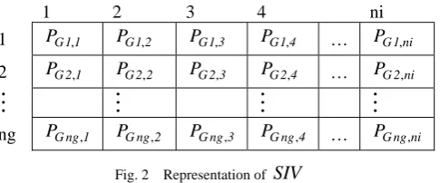
The solution process of the proposed method (PM) involves representation of problem variables and formation of a fitness function. Considering the real power generations, PG, as the problem variables, the SIVs of each island can be represented by a real number matrix as shown in Fig. 2. The variable PGit represents real power generation of unit-i at interval-
t
.1 2 3 4 ni
1 PG1,1 PG1,2 PG1,3 PG1,4 PG1,ni 2 PG2,1 PG2,2 PG2,3 PG2,4 PG2,ni
ng PGng,1 PGng,2 PGng,3 PGng,4 PGng,ni Fig. 2 Representation of SIV
The BBO searches for optimal solution by maximizing SI, like fitness function in any other stochastic optimization techniques. The SI function can be obtained by transforming the cost function into SI function as
1 1 SI
Max (12) Where is the augmented objective function, which can be formed by blending Eq. (7) with Eq. (6) through penalty factor approach as
Minimize
ni
1 t
2 ng
1 i
Lt Dt Git 2
E
1 K P P P
K
(13)
Ramp rate limits are important constraints in DEED problem. During iterative process, each SIV may
violate these constraints and represent an infeasible solution. A repair algorithm that converts an infeasible solution into a feasible one can enhance the convergence of the solution process. The proposed repair algorithm is outlined below.
1. If ramp rate constraint, given by Eq. (9) of any generator-i at interval-t violates, probabilistically choose either
P
Gi t orP
Gi t1 and replace it by a randomly generated value within its respective lowerand upper limit.
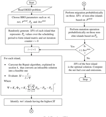
2. Repeat step-1 till the ramp rate constraints of all the generators over the scheduling period are satisfied. The solution procedure of the PM for the DEED is given through the flow chart of Fig. 3.
5. Simulation Results
Start
Read DEED problem d
Choose BBO parameters such as ni, ,
nei Pmod,Pm and Itermax
For each island,
Carryout the Repair algorithm, explained in section 4, that converts an infeasible solution into a feasible one
Evaluate
1 1 SI
Where
nt
1 t
2 ng
1 i
Lt Dt Git 2
E
1 K P P P
K
Perform migration probabilistically on those SIVs of non-elite islands
based on Pmod
Perform mutation operation probabilistically on those
non-elite islands based onPm
SIVsof the best island is the optimal solution. Compute
the net fuel cost and emissions. Is
max Iter i
? Yes
No
1
i i
Randomly generate SIVsof each island that represents PGvalues over the scheduling
period to form island matrix and set iteration counter i0
Stop
Identify nei islands having the highestSI
Fig. 3 Flow chart of PM
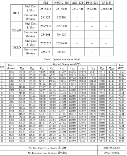
The solution of DEmD attained through setting as zero in Eq. (6), furnished in Table 3, results in the lowest emission of 284191 lb/day. The mechanism permits the system to offer the desired amount of power with smaller emissions, even smaller than that of the existing techniques. However, the DEcD and DEmD cause higher emissions of 291927 lb/day and higher fuel cost of 2655930 $/day respectively. The DEED results available in Table 4 are acquired by assigning equal to 0.5 in Eq. (1). The real power generations, fuel cost and emissions for DEED are given in Table 4. The PM attempts to lower the fuel cost, minimize emissions and extract satisfactory results in relation to those obtained by DEcD and DEmD.
Table 1 Comparison of Fuel Cost and Emissions
PM NSGA [10] AIS [13] PSO [13] EP [13]
DEcD
Fuel Cost day /
$ 2516475 2516800 2519700 2572200 2585400
Emissions day
lb/ 291927 317400 -- -- --
DEmD
Fuel Cost day /
$ 2655930 2656300 -- -- --
Emissions day
lb/ 284191 304120 -- -- --
DEED
Fuel Cost day /
$ 2522272 2522600 -- -- --
Emissions day
lb/ 285775 309940 -- -- --
Table 2 Optimal Solution for DEcD
hour Power demand
Optimal Generations (MW) Loss
(MW) 1
G
P PG2 PG3 PG4 PG5 PG6 PG7 PG8 PG9 PG10
1 1036 150.00 135.22 90.82 83.08 175.87 124.26 129.78 71.13 52.11 43.42 19.69 2 1110 150.00 135.00 137.60 62.78 178.37 158.75 129.61 87.51 49.44 43.42 22.49 3 1258 150.00 135.00 184.74 112.76 223.03 157.63 104.22 117.49 58.30 43.42 28.59 4 1406 209.38 135.00 241.01 150.26 238.35 159.93 108.48 104.41 52.06 43.42 36.30 5 1480 193.87 135.00 313.16 162.28 223.93 138.21 129.98 100.50 80.00 43.42 40.35 6 1628 219.16 194.71 337.29 201.27 204.83 147.13 129.59 120.00 80.00 43.42 49.40 7 1702 204.03 255.94 326.59 244.36 224.25 148.08 129.79 120.00 59.74 43.42 54.20 8 1776 215.10 299.41 303.67 266.94 234.23 143.70 129.83 120.00 79.31 43.42 59.61 9 1924 263.35 303.26 340.00 299.99 243.00 160.00 129.96 120.00 80.00 54.99 70.55 10 2022 336.75 336.83 340.00 300.00 243.00 160.00 130.00 120.00 80.00 55.00 79.57 11 2106 370.56 395.30 340.00 300.00 243.00 160.00 130.00 120.00 80.00 55.00 87.86 12 2150 369.73 444.72 340.00 300.00 243.00 160.00 130.00 120.00 80.00 55.00 92.44 13 2072 340.02 388.39 340.00 300.00 243.00 160.00 130.00 120.00 80.00 55.00 84.42 14 1924 279.67 345.36 308.98 273.54 242.91 160.00 129.97 120.00 79.99 54.92 71.34 15 1776 215.09 289.63 301.87 297.41 241.05 158.41 129.75 106.70 52.06 43.42 59.41 16 1554 150.00 214.28 240.96 248.41 222.99 148.35 129.78 120.00 79.93 43.42 44.13 17 1480 196.86 136.39 190.82 242.64 230.28 160.00 129.69 120.00 69.70 43.42 39.80 18 1628 234.09 216.02 211.83 254.29 227.66 160.00 129.95 120.00 80.00 43.42 49.28 19 1776 276.38 219.48 269.31 294.62 242.38 160.00 129.72 120.00 80.00 43.42 59.31 20 1972 331.06 293.77 334.34 299.99 242.96 160.00 129.93 120.00 80.00 54.99 75.04 21 1924 261.53 305.11 339.97 300.00 243.00 160.00 129.95 120.00 80.00 55.00 70.55 22 1628 208.86 225.11 261.15 288.38 224.86 123.56 129.98 120.00 52.07 43.42 49.38 23 1332 150.00 153.48 188.78 242.62 181.48 104.80 129.61 120.00 50.02 43.42 32.21 24 1184 150.00 135.00 129.64 239.19 157.24 122.92 99.62 91.68 40.74 43.42 25.45
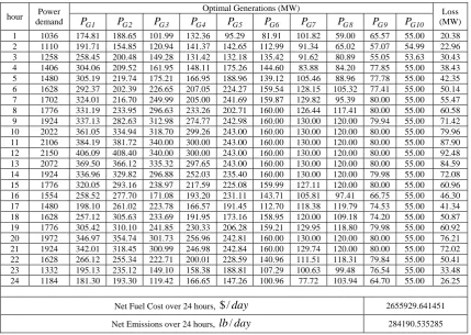
Table 3 Optimal Solution for DEmD
hour Power demand
Optimal Generations (MW) Loss
(MW) 1
G
P PG2 PG3 PG4 PG5 PG6 PG7 PG8 PG9 PG10
1 1036 174.81 188.65 101.99 132.36 95.29 81.91 101.82 59.00 65.57 55.00 20.38 2 1110 191.71 154.85 120.94 141.37 142.65 112.99 91.34 65.02 57.07 54.99 22.96 3 1258 258.45 200.48 149.28 131.42 132.18 135.42 91.62 80.89 55.05 53.63 30.43 4 1406 304.06 209.52 161.95 148.11 175.26 144.60 83.88 84.20 77.85 55.00 38.43 5 1480 305.19 219.74 175.21 166.95 188.96 139.12 105.46 88.96 77.78 55.00 42.35 6 1628 292.37 202.39 226.65 207.05 224.27 159.54 128.15 105.32 77.41 55.00 50.14 7 1702 324.01 216.70 249.99 205.00 241.69 159.87 129.82 95.39 80.00 55.00 55.47 8 1776 331.19 233.95 296.63 233.26 202.71 160.00 126.44 117.41 80.00 55.00 60.58 9 1924 337.13 282.63 312.98 274.77 242.98 160.00 130.00 120.00 79.94 55.00 71.42 10 2022 361.05 334.94 318.70 299.26 243.00 160.00 130.00 120.00 80.00 55.00 79.96 11 2106 384.19 381.72 340.00 300.00 243.00 160.00 130.00 120.00 80.00 55.00 87.90 12 2150 406.09 408.40 340.00 300.00 243.00 160.00 130.00 120.00 80.00 55.00 92.48 13 2072 369.50 366.12 335.32 297.65 243.00 160.00 130.00 120.00 80.00 55.00 84.59 14 1924 336.96 329.82 296.88 252.03 235.40 160.00 130.00 120.00 79.98 55.00 72.08 15 1776 320.05 293.16 238.97 217.59 225.08 159.99 127.11 120.00 80.00 55.00 60.96 16 1554 258.52 277.70 171.08 193.20 231.11 143.71 105.81 97.41 66.75 55.00 46.30 17 1480 198.10 261.02 223.78 166.57 191.45 112.70 118.38 119.79 74.53 55.00 41.34 18 1628 257.12 305.63 233.69 191.95 173.16 158.95 120.00 109.18 74.20 55.00 50.87 19 1776 305.42 310.10 241.85 230.33 206.28 159.21 129.95 118.80 79.98 55.00 60.92 20 1972 346.97 354.74 301.73 256.96 242.81 160.00 130.00 120.00 80.00 55.00 76.21 21 1924 342.01 318.45 300.99 246.98 242.84 160.00 129.74 120.00 80.00 55.00 72.02 22 1628 266.12 255.34 222.71 200.01 228.59 140.96 111.51 118.31 79.84 55.00 50.41 23 1332 195.13 235.12 149.10 158.38 188.81 107.29 100.63 99.48 76.54 55.00 33.48 24 1184 181.30 193.30 119.42 166.65 147.26 100.96 77.72 103.94 64.70 55.00 26.25
Net Fuel Cost over 24 hours, $/day 2655929.641451 Net Emissions over 24 hours, lb/day 284190.535285
6. Conclusion
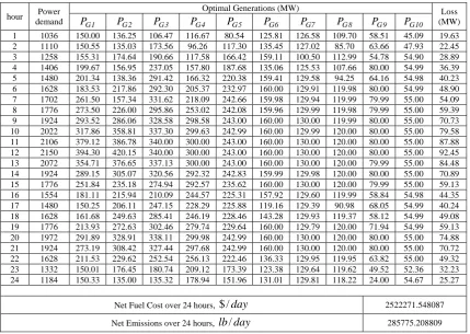
Table 4 Optimal Solution for DEED
hour Power demand
Optimal Generations (MW) Loss
(MW) 1
G
P PG2 PG3 PG4 PG5 PG6 PG7 PG8 PG9 PG10
1 1036 150.00 136.25 106.47 116.67 80.54 125.81 126.58 109.70 58.51 45.09 19.63 2 1110 150.55 135.03 173.56 96.26 117.30 135.45 127.02 85.70 63.66 47.93 22.45 3 1258 155.31 174.64 190.66 117.58 166.42 159.11 100.50 112.99 54.78 54.90 28.89 4 1406 199.67 156.95 237.05 157.80 187.68 135.06 125.53 107.66 80.00 54.99 36.39 5 1480 201.34 138.36 291.42 166.32 220.38 159.41 129.58 94.25 64.16 54.98 40.23 6 1628 183.53 217.86 292.30 205.37 232.97 160.00 129.91 119.98 80.00 54.99 48.90 7 1702 261.50 157.34 331.62 218.09 242.66 159.98 129.94 119.99 79.99 55.00 54.09 8 1776 273.50 226.00 295.86 253.02 242.08 159.96 129.99 119.98 79.99 55.00 59.39 9 1924 293.52 286.06 328.58 298.58 243.00 160.00 130.00 119.99 80.00 55.00 70.73 10 2022 317.86 358.81 337.30 299.63 242.99 160.00 129.99 120.00 80.00 55.00 79.58 11 2106 379.12 386.78 340.00 300.00 243.00 160.00 130.00 120.00 80.00 55.00 87.88 12 2150 394.30 420.15 340.00 300.00 243.00 160.00 130.00 120.00 80.00 55.00 92.45 13 2072 354.71 376.65 337.13 300.00 243.00 160.00 130.00 120.00 79.99 55.00 84.48 14 1924 289.15 305.07 320.56 292.32 242.83 159.99 129.98 120.00 80.00 55.00 70.89 15 1776 251.84 235.18 274.94 292.57 235.62 160.00 130.00 120.00 79.99 55.00 59.13 16 1554 181.11 215.94 210.09 244.57 225.31 157.92 129.60 119.99 58.84 54.98 44.35 17 1480 150.25 206.11 247.15 228.29 225.88 119.16 129.39 90.98 68.05 54.99 40.24 18 1628 161.68 249.63 285.41 246.19 228.46 143.28 129.93 119.37 58.12 54.99 49.08 19 1776 213.93 272.63 302.46 279.74 229.64 160.00 129.79 120.00 71.94 54.99 59.13 20 1972 291.89 328.91 338.11 299.98 242.99 160.00 130.00 120.00 80.00 55.00 74.88 21 1924 273.19 308.42 327.44 297.68 242.99 160.00 130.00 120.00 80.00 55.00 70.72 22 1628 211.53 229.62 252.54 256.13 222.46 136.33 129.95 119.95 63.82 55.00 49.32 23 1332 150.01 176.45 180.74 209.12 173.39 123.38 129.64 119.62 49.52 52.36 32.23 24 1184 150.33 135.00 135.32 178.94 151.96 131.01 129.81 118.22 24.00 54.67 25.27
Net Fuel Cost over 24 hours, $/day 2522271.548087 Net Emissions over 24 hours, lb/day 285775.208809
Acknowledgments
The authors gratefully acknowledge the authorities of Annamalai University for the facilities offered to carry out this work.
References
[1] Wood. AJ and Woolenberg. BF. (1996). Power generation, operation and control, John Willey and Sons, New York
[2] Chowdhury.BH and Rahman. S. (1990). A review of recent advances in economic dispatch, IEEE Trans. on Power Systems, 5(4): 1248-1259.
[3] Lamont. JW and Obessis. EV. (1995). Emission dispatch models and algorithms for the 1990’s, IEEE Trans. on Power Systems, 10(2): 941- 946.
[4] Bechert. T.E and Kwatny. H.G. (1972). On the optimal dynamic dispatch of real power, IEEE Trans. on Power Apparatus and Systems, PAS-91(3): 889-898.
[5] Xia. X, and Elaiw. A.M. (2010). Optimal dynamic economic dispatch of generation: A review, Electric Power Systems Research, 80: 975–986
[6] Hemamalini. S and Simon. S.P. (2010). Dynamic Economic Dispatch using Maclaurin Series Based Lagrangian Method, Energy Conversion and Management, 51(11): 2212-2219.
[7] Alsumait. J.S, Qasem. M, Sykulski. J.K and Al-Othman. A.K. (2010). An Improved Pattern Search Based Algorithm to Solve the Dynamic Economic Dispatch Problem with Valve-Point Effect, Energy Conversion and Management, 51(10): 2062-2067.
[8] Sivasubramani. S and Swarup. K.S. (2010). Hybrid SOA–SQP Algorithm for Dynamic Economic Dispatch with Valve-Point Effects, Energy, 35(12): 5031-5036.
[9] Panigrahi. CK, Chattopadhyah. PK, Chakrabarti. RN and Basu. N. (2006). Simulated annealing technique for dynamic economic dispatch, Electric Power Components and Systems, 34(5): 577-586.
[10]M. Basu. (2008). Dynamic economic emission dispatch using nondominated sorting genetic algorithm-II, Electrical Power and Energy Systems 30: 140–149
[11]P. Attaviriyanupap, H. Kita, E. Tanaka and J. Hasegawa. (2002). A hybrid EP and SQP for dynamic economic dispatch with non-smooth fuel cost function, IEEE Trans. on Power Systems, 17(2): 411-416.
[12]J.-. Chiou. (2009). A Variable Scaling Hybrid Differential Evolution for Solving Large-Scale Power Dispatch Problems, Generation, Transmission & Distribution, IET, 3(2): 154-163.
[13]Basu. M. (2011). Artificial Immune System for Dynamic Economic Dispatch, International Journal of Electrical Power & Energy Systems, 33(1): 131-136.
[14]Ravikumar Pandi. V and Panigrahi. B.K. (2011). Dynamic Economic Load Dispatch using Hybrid Swarm Intelligence Based Harmony Search Algorithm, Expert Syst. Appl., vol. In Press, Corrected Proof : 1-6.
[15]Simon.D. (2008). Biogeography-based optimization, IEEE Trans on Evolutionary Computation, 12(6): 702–713.
[16]P. Roy, S. Ghoshal, S. Thakur. (2010) Biogeography-based optimization for economic load dispatch problems, Electric Power Components and Systems 38, 166–181.
[17]Bhattacharya and K.P. Chattopadhyay. (2010). Solution of optimal reactive power flow using biography-based optimization, Int. Journal of Electrical and Electronics Engineering. 4(8): 568-576.
[19]A.Bhattacharya and K.P. Chattopadhyay. (2011). Application of biography-based optimization to solve different optimal power flow problems, IET Proc. Gener., Transm. & Distrib. 5(1): 70-80.
[20]S.Rajasomashekar and P. Aravindhababu. (2012). Biogeography-based optimization technique for best compromise solution of economic emission dispatch, Swarm and Evolutionary Computations, 7: 47-57.
Appendix
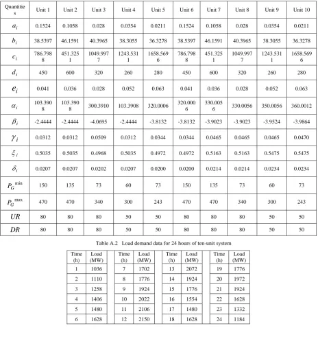
Table A.1 Ten unit system data for DEED
Quantitie
s Unit 1 Unit 2 Unit 3 Unit 4 Unit 5 Unit 6 Unit 7 Unit 8 Unit 9 Unit 10
i
a 0.1524 0.1058 0.028 0.0354 0.0211 0.1524 0.1058 0.028 0.0354 0.0211
i
b 38.5397 46.1591 40.3965 38.3055 36.3278 38.5397 46.1591 40.3965 38.3055 36.3278
i
c 786.798
8
451.325 1
1049.997 7
1243.531 1
1658.569 6
786.798 8
451.325 1
1049.997 7
1243.531 1
1658.569 6
i
d 450 600 320 260 280 450 600 320 260 280
i
e
0.041 0.036 0.028 0.052 0.063 0.041 0.036 0.028 0.052 0.063i
103.390
8
103.390
8 300.3910 103.3908 320.0006 320.000
6
330.005
6 330.0056 350.0056 360.0012
i
-2.4444 -2.4444 -4.0695 -2.4444 -3.8132 -3.8132 -3.9023 -3.9023 -3.9524 -3.9864
i
0.0312 0.0312 0.0509 0.0312 0.0344 0.0344 0.0465 0.0465 0.0465 0.0470i
0.5035 0.5035 0.4968 0.5035 0.4972 0.4972 0.5163 0.5163 0.5475 0.5475
i
0.0207 0.0207 0.0202 0.0207 0.0200 0.0200 0.0214 0.0214 0.0234 0.0234
min G
P 150 135 73 60 73 150 135 73 60 73
max G
P 470 470 340 300 243 470 470 340 300 243
UR 80 80 80 50 50 80 80 80 50 50
DR 80 80 80 50 50 80 80 80 50 50
Table A.2 Load demand data for 24 hours of ten-unit system
Time (h)
Load (MW)
Time (h)
Load (MW)
Time (h)
Load (MW)
Time (h)
Load (MW)
1 1036 7 1702 13 2072 19 1776
2 1110 8 1776 14 1924 20 1972
3 1258 9 1924 15 1776 21 1924
4 1406 10 2022 16 1554 22 1628
5 1480 11 2106 17 1480 23 1332
6 1628 12 2150 18 1628 24 1184
Table A.3 B-loss coefficients for ten unit system data
0.000014 0.000045 0.000016 0.000016 0.000017 0.000015 0.000015 0.000016 0.000018 0.000018
0.000015 0.000016 0.000039 0.000010 0.000012 0.000012 0.000014 0.000014 0.000016 0.000016
0.000015 0.000016 0.000010 0.000040 0.000014 0.000010 0.000011 0.000012 0.000014 0.000015
0.000016 0.000017 0.000012 0.000014 0.000035 0.000011 0.000013 0.000013 0.000015 0.000016
0.000017 0.000015 0.000012 0.000010 0.000011 0.000036 0.000012 0.000012 0.000014 0.000015
0.000017 0.000015 0.000014 0.000011 0.000013 0.000012 0.000038 0.000016 0.000016 0.000018
0.000018 0.000016 0.000014 0.000012 0.000013 0.000012 0.000016 0.000040 0.000015 0.000016
0.000019 0.000018 0.000016 0.000014 0.000015 0.000014 0.000016 0.000015 0.000042 0.000019