FUZZY MULTINOMIAL CONTROL
CHART WITH VARIABLE SAMPLE
SIZE
A. PANDURANGAN
Professor and Head
Department of Computer Applications
Valliammai Engineering College, Kattankulathur, Chennai – 603 203, India. e-mail id : [email protected]
R. VARADHARAJAN
Assistant Professor in Statistics Department of Management Studies
VELS University, Pallavaram, Chennai – 600 117, India e-mail id: [email protected]
Abstract:
The control chart technique is being widely used in industries to monitor a process for quality improvement. One of the basic charts for attributes is the p-chart. For a p – chart each item is classified as either nonconforming or conforming to the specified quality characteristic. In Some cases, an item may be classified in more than two categories such as “bad”, “medium”, “good”, and “excellent”. Based on this concept, Amirzadeh et al. [1] have developed Fuzzy Multinomial chart (FM-chart) with the fixed sample size (FSS). In this paper a Fuzzy Multinomial process with Variable Sample Size (VSS) is proposed and the control limits for the FM chart have been obtained using multinomial distribution. The proposed method is compared with the conventional p – chart. It is seen that FM chart with VSS performs better than the conventional chart.
Key words: Multinomial distribution; FM-chart; p–chart; Variable sample size; Linguistic variable; Membership function; Fuzzy statistics.
1. Introduction:
Statistical Process Control (SPC) is used to monitor the process stability which ensures the predictability of the process. The power of control charts lies in their ability to detect process shift and to identify abnormal condition in the process. In 1924, Walter Shewhart designed the first control chart as follows: Let w be a sample statistic that measures some quality characteristic of interest and suppose that the mean of w is µw and the standard deviation of w is σw. Then the center line (CL), the upper control limit (UCL) and the
lower control limit (LCL) are defined as
UCL = µw + d σw CL = µw LCL = µw – d σw
where d is the “distance” of the control limits from the center line, expressed in standard deviation units.
2. Fuzzy logic and Linguistic variables:
The concept of fuzzy logic plays a fundamental role in formulating quantitative fuzzy variables. These are variables whose states are fuzzy members. The members represent linguistic concepts, such as very small, small, medium and so on, as interpreted in a particular context. The resulting constructs are usually called linguistic variables. The linguistic terms are commonly used in industry to express properties or characteristics of a particular product.
The conformity to specifications on a quality standard is evaluated onto a two-state scale, for example, acceptable or unacceptable, good or bad, and so on. In some situations the binary classification might not be suitable, where product quality can assume more intermediate states. The assignment of weights, to reflect the degree of severity of product nonconformity has been adopted in many circumstances. When the products are classified into mutually exclusive linguistic categories, fuzzy control charts are used. Different procedures are proposed to construct these charts. Raz and Wang [7,10] developed fuzzy control charts for linguistic data which are mainly based on membership and probabilistic approaches.
In this paper, a fuzzy multinomial control chart (FM chart) for linguistic variables with variable sample size is proposed. The FM – chart deals with a linguistic variable which is classified into more than two categories. The FM – chart with VSS found to be more effective than p – chart for studying the shift in process mean.
3. Methodology:
Based upon Fuzzy set theory, a linguistic variable
L
~
is characterized by the set of k mutually exclusive members{
l
1,
l
2...
l
k}
. We attach a weightm
i to each terml
i that reflects the degree of membershipin the set. Then it can be written by a fuzzy set as
L
~
=
{
(
l
1,
m
1),
(
l
2,
m
2),...(
l
k,
m
k)
}
. . . (1).To monitor the out of control signal in the production process take independent samples of different sizes. The size of the sample to be drawn each time is decided by choosing a member randomly from
{
n
1,
n
2,...
n
s}
.
4. Fuzzy Multinomial Control Chart:
In this section a new approach for construction of Fuzzy multinomial control chart based on variable sample size is proposed. The statistical principles underlying the fuzzy multinomial control chart (FM -chart) with variable sample size are based on the multinomial distribution.
As defined in (1),
L
~
is a linguistic variable which can take k mutually exclusive members{
l
1,
l
2...
l
k}
.Assume that the production process is operating in a stable manner and
p
i is the probability that an item isl
i, i= 1, 2 …k. and successive items produced are independent. Suppose that a random sample of size
n
r units ofthe product is selected and let
X
i, i = 1, 2 …k, be the number of items of the product that arel
i, i = 1, 2 …k. Then{
X
1,
X
2...
X
k}
has a multinomial distribution with parametersn
r andp
1,
p
2...
p
k. It is known that eachX
i, i = 1, 2 …k, marginally has a binomial distribution with the meann
rp
i and variancen
rp
i(
1
−
p
i)
, i = 1, 2 …k, respectively. The weighted average of the linguistic variableL
~
with sample sizen
r is defined by
= =
=
ki i
i k
i i
X
m
X
L
1 1
~
=
r i k
i i
n
m
X
=1
,
n
r∈
{
n
1,
n
2,...
n
s}
. . . (2)The control limits for FM – chart are
5. Theorem:
Let
L
~
=
{
(
l
1,
m
1),
(
l
2,
m
2),...(
l
k,
m
k)
}
be a linguistic variable such thatp
i is the probability that anitem is
l
i, i = 1, 2, …k. IfX
i, i = 1, 2 …k is the number of units of the product that arel
i, i = 1, 2 …k in a sample of sizen
r, then(i)
E
[
L
~
]
= ik i i
m
p
=1(ii)
var(
L
~
)
=
−
−
< = = = k j i i k j j i j i i i k i i rp
p
m
m
p
p
m
n
1 1 12
)
2
)
1
(
1
,
n
r∈
{
n
1,
n
2,...
n
s}
where
n
1,
n
2,...
n
s are pre-determined sample sizes.Proof:
In a sample of
n
r units,X
i has a binomial distribution with the meann
rp
i and variance)
1
(
ii r
p
p
n
−
, i = 1, 2, …k andCov (
X
i,X
j) =−
n
rp
ip
j, ifi
≠
j
and then(i) The mean is:
E
[
L
~
]
=
= r k i i in
X
m
E
1 = r k i i in
X
E
m
=1)
(
= r k i i r in
p
n
m
=1= i k i i
m
p
=1,
n
r∈
{
n
1,
n
2,...
n
s}
. . . (3)(ii) The variance is:
var(
L
~
)
=
= r k i i in
X
m
1var
=
=)
var(
1
1 2 k i i i rX
m
n
,=
1
2[
var(
1 1 2 2...
k k)
]
r
x
m
x
m
x
m
n
+
+
+
=
+
< = = =)
,
cov(
2
)
var(
1
1 1 1 22 i j
k j i i k j j i i k i i r
X
X
m
m
X
m
n
=
+
< = = =)
,
cov(
2
)
var(
1
1 1 1 22 i j
k j i i k j j i i k i i r
X
X
m
m
X
m
n
=
−
+
−
< = = = k j i i k j j i r j i i i r k i i rp
p
n
m
m
p
p
n
m
n
1 1 12
2
(
1
)
2
(
)
1
=
−
−
< = = = k j i i k j j i j i i i k i i rp
p
m
m
p
p
m
n
1 1 12
)
2
)
1
(
1
, where
n
r∈
{
n
1,
n
2,...
n
s}
. . . . (4)6. Choice of Sample size:
Many authors, for example [2], [8] have recommended variable sample sizes (VSS) for the construction of control charts for variables as well as attributes. Later, the Markov dependent sample size (MDSS) was proposed by Sivasamy et al [9], and Pandurangan [6] for the advantage of economic sampling inspection. Now, to construct FM control chart the sample size for each draw can be randomly chosen from the pre – determined set
{
n
1,
n
2,...
n
s}
. The advantage of taking variable sample size lies in ASN and consequently the costs of sampling inspection.7. Numerical Example:
On a production line, a visual control of the aluminum die-cast of a lighting component might have the following assessment possibilities
1. "reject" if the aluminum die-cast does not work;
2. "poor quality" if the aluminum die-cast works but has some defects;
3. "medium quality" if the aluminum die-cast works and has no defects, but it has some aesthetic flaws; 4. "good quality" if the aluminum die-cast works and has no defects, but has few aesthetic flaws;
5. "excellent quality" if the aluminum die-cast works and has neither defects nor aesthetic flaws of any kind. To monitor the quality of this product, 25 samples of different sizes are selected. The degrees of membership for the above assessment are taken as 1, 0.75, 0.5, 0.25 and 0 respectively. The data with
L
i~
and
i
p
ˆ
are given in Table – 1.The value of
L
i~
can be calculated to the following ways
= =
=
ki i
i k
i i i
X
m
X
L
1 1
~
=
r i k
i i
n
m
X
=1
,
n
r∈
{
n
1,
n
2,...
n
s}
{
}
0
.
390
100
)
0
12
(
)
25
.
0
54
(
)
5
.
0
12
(
)
75
.
0
10
(
)
1
12
(
~
1
=
×
+
×
+
×
+
×
+
×
=
L
{
}
0
.
372
80
)
0
8
(
)
25
.
0
48
(
)
5
.
0
9
(
)
75
.
0
7
(
)
1
8
(
~
2
=
×
+
×
+
×
+
×
+
×
=
L
{
}
0
.
388
80
)
0
8
(
)
25
.
0
43
(
)
5
.
0
12
(
)
75
.
0
11
(
)
1
6
(
~
3
=
×
+
×
+
×
+
×
+
×
=
L
And so on, and the value of
p
ˆ
i, the control limits for p – charts can be calculated as followsr i i
n
D
p
ˆ
=
,n
r∈
{
n
1,
n
2,...
n
s}
0
.
120
100
12
ˆ
1 1
1
=
=
=
n
D
p
,0
.
100
80
8
ˆ
2 2
2
=
=
=
n
D
p
,0
.
075
80
6
ˆ
3 3
3
=
=
=
n
D
p
; and soTable – 1
Sample No
Sample
size Reject®
Poor Quality(PQ)
Medium Quality(MQ)
Good Quality(GQ)
Excellent
Quality(EQ)
L
i~
i
p
ˆ
1 100 12 10 12 54 12 0.390 0.120
2 80 8 7 9 48 8 0.372 0.100
3 80 6 11 12 43 8 0.388 0.075
4 100 9 7 13 53 18 0.340 0.090
5 110 10 16 18 54 12 0.405 0.091
6 110 12 5 17 60 16 0.357 0.109
7 100 11 12 13 50 14 0.390 0.110
8 100 10 22 18 45 5 0.468 0.100
9 90 10 8 13 50 9 0.389 0.111
10 90 6 5 14 51 14 0.328 0.067
11 110 20 13 23 47 7 0.482 0.182
12 120 15 13 20 58 14 0.410 0.125
13 120 9 12 22 64 13 0.375 0.075
14 120 8 9 20 61 22 0.333 0.067
15 110 6 10 19 61 14 0.348 0.055
16 80 8 5 12 47 8 0.369 0.100
17 80 10 8 12 40 10 0.400 0.125
18 80 7 13 10 42 8 0.403 0.088
19 90 5 7 14 54 10 0.342 0.056
20 100 8 11 14 50 17 0.358 0.080
21 100 5 8 16 58 13 0.335 0.050
22 100 8 9 15 51 17 0.350 0.080
23 100 10 12 14 50 14 0.385 0.100
24 90 6 13 17 45 9 0.394 0.067
25 90 9 10 14 46 11 0.389 0.100
The control limits for p – chart is obtained as follows
096
.
0
2450
234
1
1
=
=
=
= =
s
r r k
i i
n
D
p
For Sample 1:
0
.
184
100
)
096
.
0
1
(
096
.
0
3
096
.
0
)
1
(
1
=
−
+
=
−
+
=
r
n
p
p
d
p
UCL
096
.
0
1
=
p
=
CL
;008
.
0
100
)
096
.
0
1
(
096
.
0
3
096
.
0
)
1
(
1
=
−
−
=
−
−
=
r
n
p
p
d
p
LCL
,For Sample 2:
0
.
195
80
)
096
.
0
1
(
096
.
0
3
096
.
0
)
1
(
2
=
−
+
=
−
+
=
r
n
p
p
d
p
UCL
096
.
0
2
=
p
=
CL
;003
.
0
80
)
096
.
0
1
(
096
.
0
3
096
.
0
)
1
(
2
=
−
−
−
=
−
−
=
r
n
p
p
d
p
LCL
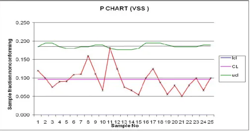
,Fig. 1: The p – chart for the 25 samples.
In Figure 1, the out of control signal is seen corresponding to 11th sample, for which the sample size is 110. From the p – chart, out of 2450 sample observations, 1070 sample observations were needed to get the signal. The corresponding center line and control limits are as under
CL = 0.096, UCL = 0.180 and LCL = 0.012
To construct the FM – chart, the UCL and LCL values are computed for each sample as follows
For Sample 1:
)
~
var(
]
~
[
1 11
E
L
d
L
UCL
=
+
i k
i i
m
p
=
=
1+
−
−
<
= =
=
k
j i i
k
j
j i j i i
i k
i
i
p
p
m
m
p
p
m
n
d
1 1 1
2
1
)
2
)
1
(
1
=
0
.
3750
+
3
0
.
0008214
=
0
.
4609
[
~
]
0
.
3750
1 1
1
=
=
=
=
m
p
L
E
CL
k
i i
)
~
var(
]
~
[
1 11
E
L
d
L
LCL
=
−
i
k
i i
m
p
=
=
1-
−
−
<
= =
=
k
j i i
k
j
j i j i i
i k
i
i
p
p
m
m
p
p
m
n
d
1 1 1
2
1
)
2
)
1
(
1
=
0
.
3750
−
3
0
.
0008214
=
0
.
2891
For Sample 2:
)
~
var(
]
~
[
2 22
E
L
d
L
i
k
i i
m
p
=
=
1+
−
−
<
= =
=
k
j i i
k
j
j i j i i
i k
i
i
p
p
m
m
p
p
m
n
d
1 1 1
2
2
)
2
)
1
(
1
=
0
.
3863
+
3
0
.
001234
=
0
.
4917
[
~
]
0
.
3863
1 2
2
=
=
=
=
m
p
L
E
CL
k
i i
)
~
var(
]
~
[
2 22
E
L
d
L
LCL
=
−
i
k
i i
m
p
=
=
1-
−
−
<
= =
=
k
j i i
k
j
j i j i i
i k
i
i
p
p
m
m
p
p
m
n
d
1 1 1
2
2
)
2
)
1
(
1
=
0
.
3863
−
3
0
.
001234
=
0
.
2809
, and so on.FM – chart for the 25 samples is given in Figure 2.
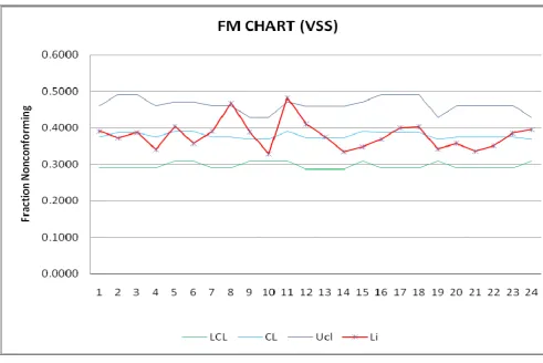
Fig. 2: The FM – chart for the 25 samples.
Figure 2 shows that the process is out of control at samples 8 and 11, the respective sample sizes are 100 and 110 and the corresponding center lines and control limits are
(i) CL = 0.3750, UCL = 0.4609 and LCL = 0.2891 for sample size 100. (
P
R = 0.10,P
PQ = 0.22,P
MQ = 0.18,P
GQ = 0.45,P
EQ = 0.05) (ii) CL = 0.3898, UCL = 0.4710 and LCL = 0.3086 for sample size 110.be inspected to get the alarm with the help of a p – chart. Thus, the FM is more economical and more sensitive in identifying any shift in the specified quality level.
Conclusion:
FM – chart has been proposed for linguistic data set. To draw the chart, samples of varying sizes are chosen randomly from a pre–determined set. The FM-chart has been compared with the conventional p–chart with VSS. It is shown that the FM – chart is more economical and more sensitive in giving the alarm for shift in the specified quality level. This work can be extended for Markov dependent sample sizes.
REFERENCES
[1] Amirzadeh, V.; M. Mashinchi; M.A. Yaghoobi. (2008). Construction of Control Charts Using Fuzzy Multinomial Quality.Journal of Mathematics and Statistics 4 (1): pp.26-31.
[2] Costa A.F.B, (1994). “
X
-chart with variable sample size”. Journal of Quality Technology, 26, pp. 155-163.[3] Franceschini, F. and D. Romano, (1999). Control chart for linguistic variables: A method based on the use of linguistic quantifiers. International Journal of Production Research. 37: pp. 3791-3801.
[4] Gulbay, M., C. Kahraman and D. Ruan, (2004). α - cut fuzzy control charts for linguistic data. International Journal of Intelligent Systems. 19: pp.1173-1196.
[5] Kanagawa, A., F. Tamaki and H. Ohta, (1993).Control charts for process average and variability based on linguistic data. International Journal of Production Research. 31:pp. 913-922.
[6] Pandurangan A., (2002). “Some Applications of Markov Dependent Sampling Scheme in SQC”, Unpublished Ph.D Thesis, Bharathidasan University, Tiruchirappalli,
[7] Raz, T. and J.H. Wang, (1990). Probabilistic and membership approaches in the construction of control charts for linguistic data. Production Planning and Control. J. Math. & Stat. 4 (1): 26-31, 2008 31.
[8] Sawlapurkar, U, Reynolds, M.R.Jr, Arnold, J.C (1990). “Variable Sample Size
X
-charts”. Presented at the winter conference of the American Statistical Association, Orlando, FL.[9] Sivasamy, R, Santhakumaran, A and Subramanian, C (2000). “Control charts for Markov Dependent Sample Size”. Quality Engineering, 12(4), pp. 596-601.