Ocean Sci., 15, 1627–1651, 2019 https://doi.org/10.5194/os-15-1627-2019 © Author(s) 2019. This work is distributed under the Creative Commons Attribution 4.0 License.
Vertical structure of ocean surface currents under high winds from
massive arrays of drifters
John Lodise1, Tamay Özgökmen1, Annalisa Griffa2, and Maristella Berta2
1RSMAS, University of Miami, Department of Ocean Sciences, Miami, FL 33149, USA 2CNR-ISMAR, Department of Physical and Chemical Oceanography, Lerici, Italy
Correspondence:John Lodise ([email protected]) Received: 28 February 2019 – Discussion started: 5 March 2019
Revised: 21 October 2019 – Accepted: 22 October 2019 – Published: 9 December 2019
Abstract. Very-near-surface ocean currents are dominated by wind and wave forcing and have large impacts on the transport of buoyant materials in the ocean. Surface currents, however, are under-resolved in most operational ocean mod-els due to the difficultly of measuring ocean currents close to, or directly at, the air–sea interface with many modern in-strumentations. Here, observations of ocean currents at two depths within the first meter of the surface are made utiliz-ing trajectory data from both drogued and undrogued Con-sortium for Advanced Research on Transport of Hydrocar-bon in the Environment (CARTHE) drifters, which have draft depths of 60 and 5 cm, respectively. Trajectory data of dense, colocated drogued and undrogued drifters were collected during the Lagrangian Submesoscale Experiment (LASER) that took place from January to March of 2016 in the northern Gulf of Mexico. Examination of the drifter data reveals that the drifter velocities become strongly wind- and wave-driven during periods of high wind, with the pre-existing regional circulation having a smaller, but non-negligible, influence on the total drifter velocities. During these high wind events, we deconstruct the total drifter velocities of each drifter type into their wind- and wave-driven components after subtracting an estimate for the regional circulation, which pre-exists each wind event. In order to capture the regional circulation in the absence of strong wind and wave forcing, a Lagrangian varia-tional method is used to create hourly velocity field estimates for both drifter types separately, during the hours preceding each high wind event. Synoptic wind and wave output data from the Unified Wave INterface-Coupled Model (UWIN-CM), a fully coupled atmosphere, wave and ocean circula-tion model, are used for analysis. The wind-driven compo-nent of the drifter velocities exhibits a rotation to the right
with depth between the velocities measured by undrogued and drogued drifters. We find that the average wind-driven velocity of undrogued drifters (drogued drifters) is ∼3.4 %– 6.0 % (∼2.3 %–4.1 %) of the wind speed and is deflected ∼5–55◦(∼30–85◦) to the right of the wind, reaching higher deflection angles at higher wind speeds. Results provide new insight on the vertical shear present in wind-driven surface currents under high winds, which have vital implications for any surface transport problem.
1 Introduction
a wide range of parameterizations of wind-driven dynamics over relatively deep surface layers, forced with climatologi-cal winds (Chassignet et al., 2003, 2007).
Observational data that capture the vertical shear within the first meter of wind-driven surface currents are very ited in the real ocean as well. This is mainly due to the lim-itations of the instrumentation used to gather these physical data. The majority of Lagrangian drifter studies have used classic drifter designs, namely CODE and Surface Velocity Program (SVP) drifters (Davis, 1985; Lumpkin and Pazos, 2007), that span depths ranging from 1 to 30 m (Lumpkin et al., 2017) and are therefore unrepresentative of the wind forced current at the very surface. Santala and Terray (1992) describe the difficulty in measuring surface velocities, as well as near-surface shear, due to wave bias present when uti-lizing any instrumentation whose motion is dependent on wave action. Acoustic Doppler current profilers (ADCPs) are not able to accurately measure velocities near an undu-lating boundary, making it difficult to sample surface layers above depths of 0.5 m (Cole and Symonds, 2015; Sentchev et al., 2017). High-frequency (HF) radars, excluding those with multi-frequency capabilities, are known to measure vertically integrated surface currents, with about 80 % of the radar sig-nal originating in the upper 1 m, depending on the electro-magnetic frequency (∼16 MHz) of the radar, such that ver-tical shear within this depth is not detectible in the measure-ment (Stewart and Joy, 1974; Rohrs et al., 2015). Some work, however, has shown promise in detecting vertical shear by calculating Doppler shifts from multiple Bragg wave peaks simultaneously (Ivonin et al., 2004).
Using a novelty suite of instruments in the Gulf of Mex-ico, Laxague et al. (2018) observed wind- and wave-induced surface currents within 1 cm of the surface, under low winds (U10=4 m s−1), to be twice as fast as the average current over the first 1 m and 4 times as fast as the average current over the upper 10 m (the upper 10 m average being equal to ∼0.16 m s−1). Another study using drifters of multiple draft depths and HF radar data led to a similar result, showing that HF radar velocity measurements taken at∼2–3 m depth, were, on average, only 55.7 % of that measured with ultra-thin drifters with 5 cm draft depths, whose absolute velocity was on the order of 0.3 m s−1(Morey et al., 2018). Compari-son of surface velocities measured with ultra-thin drifters of 5 and 10 cm draft depths also showed a rapid decay of velocity away from the surface, with the 10 cm drifters traveling 10 % slower on average (Morey et al., 2018). The sharp change in wind- and wave-induced velocities observed in these two studies reveals the need for increased vertical resolution of these surface measurements (Laxague et al., 2018; Morey et al., 2018).
Classical Ekman theory states that wind-driven currents at the very surface travel at a deflection angle of 45◦to the right of the wind in the Northern Hemisphere, when one assumes a balance between Coriolis and friction under stationary, ho-mogeneous conditions (Ekman, 1905). Laboratory studies
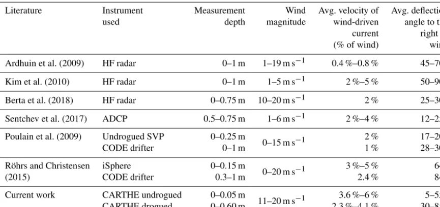
have shown that total surface drift currents induced by wind and waves combined travel at∼3.1 % of the wind velocity, with the wind-induced drift decreasing and the wave-induced drift increasing, with increasing fetch (Wu, 1983). Various observational studies on wind-driven currents over the up-per∼1 m of the surface, which utilized a range of different instruments including HF radars, ADCPs and drifters of var-ious types (i.e. CODE, iSphere or undrogued SVP drifters), have reported a wide range of deflection angles ranging from 15 to 90◦ to the right of the wind at varying wind speeds (Ardhuin et al., 2009; Poulain et al., 2009; Kim et al., 2010; Röhrs and Christensen, 2015; Sentchev et al., 2017; Berta et al., 2018). Individual results and details of these studies are presented in Table 1. Combined results of these stud-ies produce a range of estimates for the magnitude of wind-induced currents, with reported values ranging from 0.4 % to 5 % of the wind velocity, over the upper∼1 m, showing that results may vary significantly based on environmental conditions and methodology (Ardhuin et al., 2009; Poulain et al., 2009; Kim et al., 2010; Röhrs and Christensen, 2015; Sentchev et al., 2017; Berta et al., 2018). Changes in upper ocean stratification and mixed layer depth have been shown to have large effects on the deflection angle and relative ve-locity of surface currents with respect to the wind (Kudryavt-sev and Soloviev, 1990; Sutherland et al., 2016). Rascle and Ardhuin (2009) showed how the complicated relationship be-tween wave-induced mixing and varying stratification can re-sult in quasi-Eulerian wind-driven surface currents ranging from∼1 % to 3 % of the wind speed, having deflection an-gles ranging from∼35 to 90◦.
J. Lodise et al.: Vertical structure of ocean surface currents 1629
Table 1.Review of literature on wind-driven surface currents using real ocean, observational data.
Literature Instrument Measurement Wind Avg. velocity of Avg. deflection
used depth magnitude wind-driven angle to the
current right of
(% of wind) wind
Ardhuin et al. (2009) HF radar 0–1 m 1–19 m s−1 0.4 %–0.8 % 45–70◦
Kim et al. (2010) HF radar 0–1 m 1–5 m s−1 2 %–5 % 50–90◦
Berta et al. (2018) HF radar 0–0.75 m 10–20 m s−1 2 % 25–30◦
Sentchev et al. (2017) ADCP 0.5–0.75 m 1–6 m s−1 2 %–4 % 12–25◦
Poulain et al. (2009) Undrogued SVP 0–0.25 m
0–15 m s−1 2 % 17–20
◦
CODE drifter 0–1 m 1 % 28–30◦
Röhrs and Christensen iSphere 0–0.15 m
0–20 m s−1 3 %–5 % 64
◦
(2015) CODE drifter 0.3–1 m 2.4 % 84◦
Current work CARTHE undrogued 0–0.05 m
11–20 m s−1 3.6 %–6 % 5–55
◦
CARTHE drogued 0–0.60 m 2.3 %–4.1 % 30–85◦
Upon inspection of the total velocity of the drifters dur-ing the high wind events, we hypothesize that there are three dominant components that drive the drifter velocities: a wind-driven component, a wave-driven component and the regional circulation that pre-existed each high wind event. Assuming a simple linear superposition of the velocity com-ponents, we define the total velocity of each drifter type as the depth-averaged integral:
¯ uT=
1
h
h
Z
0
[us(z)+uw(z)+urc(z)] dz, (1)
whereuwis the purely wind-driven velocity,usis the Stokes
drift velocity,urcis the regional circulation that exists before
the increase in synoptic winds,zis the depth being evaluated, andhis the draft depth of the respective drifter. Given this definition of the total drifter velocities, we neglect possible nonlinear interactions between velocity components, which will be considered in future investigations.
The three components in Eq. (1) were estimated as fol-lows:us was calculated numerically with the Unified Wave
INterface-Coupled Model (UWIN-CM; Chen et al., 2013) during the LASER campaign and stored for later analysis, urcis estimated from the dense population of drifters in the
region in the hours preceding substantial increases in syn-optic winds using Lagrangian variational analysis (LAVA; Taillandier et al., 2006) to create Eulerian velocity fields of the regional circulation, and we solve foruwby subtracting
the estimated regional circulation and Stokes drift velocity from the total velocity of the drifters. To evaluate the perfor-mance of the LAVA-derived velocity fields, we use Aviso sea surface temperature (SST) and absolute geostrophic velocity products, in addition to ocean current velocity fields from the Navy Coordinate Ocean Model (NCOM) for comparison.
In the northwestern Mediterranean Sea, the underlying geostrophic currents were shown to retain their structure and influence the surface flow under high wind forcing for time periods on the order of 2–3 d (Berta et al., 2018). In the present study, the timescales over which the flow fea-tures of the regional circulation,urc, retain their structure
un-der strong winds are difficult to determine given the current dataset. However, the subtraction of the pre-existing regional circulation from the total velocity of the drifters during the high wind events shows a posteriori that the pexisting re-gional circulation retains its structure, to a reasonable extent, during the high wind analysis periods on which we focus. Af-ter subtracting the pre-existing regional circulation and nu-merically calculated Stokes drift velocity,us, from the full
velocity of the drifters,u¯T, during each period of high wind, we are left with an estimate for the average, purely wind-driven component,uw, of each drifter type.
The paper is organized as follows: Sect. 2 describes the CARTHE drifters, the configuration of UWIN-CM and NCOM, and the Aviso data products. Section 3 explains LAVA used to create the estimated Eulerian velocity fields of the pre-existing regional circulation, as well as the cal-culations involved in the deconstruction of the total drifter velocities,u¯T, along each drifter trajectory during the high
2 Data
2.1 CARTHE drifter
The CARTHE drifter is a biodegradable surface drifter that consists of a Spot Trace GPS unit by Global Star, a torus float which contains the GPS housing, two interlocking panels that form the drogue and a flexible rubber tube that connects the drogue and float (Novelli et al., 2017). During the LASER experiment, over 1000 CARTHE drifters were deployed with drogues; however, over the first 7 weeks of the experiment, approximately 40 % of the drifters lost their drogues (Haza et al., 2018). Drogued and undrogued drifters have draft depths of 60 and 5 cm, respectively, and have been extensively ana-lyzed with respect to their specific drift characteristics during laboratory experiments performed by Novelli et al. (2017). For this study, a subset of colocated drogued and undrogued drifters from the LASER campaign is used for analysis, due to their opportunistic location during the passage of large at-mospheric fronts across the northern Gulf of Mexico.
Drogue loss during the experiment mostly coincided with large storm and wave events and the precision of the deter-mined time of drogue loss was 0.5 to 3 h for 85 % of the drifters (Haza et al., 2018). The method for drogue loss de-tection is based on the differential velocities of the drifters, as the undrogued drifters are preferentially accelerated by the higher velocities of wind- and wave-driven currents present in the shallower surface layer in which the undrogued drifters reside. In addition, undrogued drifters display a decreased, more sporadic GPS transmission rate, due to their tendency to be flipped by large or breaking waves, which points the GPS antennae downwards and reduces the ability of the GPS to transmit until the drifter is flipped upright again. Despite this, 80 % of the time intervals between transmissions by un-drogued drifters are still between 4.5 and 5.5 min, but with notably higher outliers than the drogued drifters (Haza et al., 2018). The algorithm for drogue detection used by Haza et al. (2018) was validated using a subset of 50 drifters with known drogue status and was shown to distinguish drogued and undrogued drifters with an accuracy of 94 %–100 %. This very successful drogue detection algorithm has pro-vided the opportunity to utilize both drogued and undrogued drifters to study the variation of very-near-surface currents with depth (Haza et al., 2018).
GPS transmissions reported each drifter’s location every 5 min during the experiment with an accuracy of about 7 m. In addition to the extensive categorization of drogued and undrogued drifters, the drifter trajectory data were also qual-ity controlled for missing transmissions and linearly inter-polated to regular 15 min intervals (Haza et al., 2018). Ve-locities were then calculated, resulting in estimates for the average velocity of each drifter over 15 min intervals.
When using drifters to study ocean currents, concerns about different sources of velocity slip must be ad-dressed. Extensive laboratory testing performed by Novelli
et al. (2017) using half-scale drogued and undrogued drifters showed that in the absence of wind and waves drogued (un-drogued) drifters travel within 0.01 m s−1(0.02 m s−1) of the mean Eulerian current averaged over the draft depth of the given drifter. Under the effects of waves, observed in the ab-sence of wind, the undrogued drifter unsurprisingly feels an acceleration due to Stokes drift, but the drogued drifter feels a reduced wave-induced acceleration due to the flexible tether holding together its float and drogue. This mechanical decou-pling partially removes the effect of the Stokes drift acting on the drogued drifter, mainly dampening the effects of Stokes drift above the drogue (Novelli et al., 2017).
To characterize the slip velocity associated with wind, waves and Eulerian current, Novelli et al. (2017) defines the “absolute” slip velocity as the difference between the veloc-ity of a drifter and the depth-integrated current over each drifters’ draft. The absolute slip velocity of both drogued and undrogued drifters during laboratory testing was found to decrease with increasing wind speed, decreasing from 3 to 0.1 cm s−1for the drogued drifter and from 14 to 1 cm s−1for the undrogued drifter, for wind speeds from 8.1 to 23 cm s−1. This phenomenon is thought to be caused by wind separa-tion from the ocean surface due to the presence of surface gravity waves (Novelli et al., 2017). Another laboratory ex-periment, focused on measuring the turbulent air flow over wind generated waves in a similar wind-wave tank, found wind separation to occur over 90 % of short wind waves at 10 m wind speeds of∼16 m s−1(Buckley and Veron, 2017). The extent to which wind separation occurs and its effec-tiveness of sheltering the drifters from wind slip in the real ocean is difficult to quantify given the scale differences be-tween the laboratory wave tank and open ocean. However, another recent experiment using full-size CARTHE drogued and undrogued drifters in the real ocean, alongside a suite of instruments including an ADCP and polarimetric camera, showed that velocities calculated using both drifter types fell within the range of velocities measured by other instrumen-tation over the corresponding draft of each drifter (Laxague et al., 2018). Because the extent to which velocity slip affects the drifters in the real ocean is not well known during high wind and wave conditions, we chose not to attempt a correc-tion of the drifter velocities to account for such measurement errors.
2.2 UWIN-CM
J. Lodise et al.: Vertical structure of ocean surface currents 1631
over the Gulf of Mexico with 36 vertical layers (Skamarock et al., 2008; Haza et al., 2018).
The surface gravity wave model is the University of Mi-ami Wave Model v2 (UMWM; Donelan et al., 2012), with the same 4 km resolution as the atmospheric component. The three-dimensional Stokes drift velocity fields are calculated as the full integral:
us=
2π
Z
0 kmax Z
kmin
ωk2cosh [2k (d+z)]
2sinh2kd F (k, θ )dkdθ, (2)
where ωis the angular frequency, k is the wavenumber,d
is the mean water depth,zis the depth being evaluated,F
is the wavenumber energy spectrum, and θ is the direction of the waves (Stokes, 1847; Phillips, 1977). Over the en-tirety of LASER,kranged from 0.0039 to 16.0739 rad m−1, in 37 logarithmic increments, which corresponds to a range of wavelengths from 1611 to 0.39 m, respectively. The Hy-brid Coordinate Ocean Model (HYCOM) v2.2 is used as the ocean circulation model; however, no model output from this circulation model is used for the analysis of wind-driven cur-rents. The surface layer of the HYCOM model has a mini-mum thickness of 3 m, which makes the model unrepresen-tative of the depths sampled by the drifters and very difficult to validate with observational data (Wallcraft et al., 2009). Comparison of drifter data and surface velocities from the circulation model showed obvious discrepancies at the spa-tial scales necessary for this study.
The coupling between the model components is as fol-lows: WRF passes radiative and heat fluxes, as well as precip-itation rates to the ocean model, as well as the air density and wind profiles to the wave model. The wave model (UMWM) passes vectorial atmosphere stress and vectorial ocean stress to the atmosphere model and ocean circulation model, re-spectively. The ocean circulation model passes SST to the at-mosphere model and surface current fields and ocean density to the wave model. WRF and UMWM fields are exchanged every 60 s, while HYCOM fields are exchanged every 120 s (Chen and Curcic, 2016b).
The UWIN-CM is initialized daily using initial and bound-ary conditions from Global Forecast System (GFS) and global HYCOM fields along with the previous day’s UMWM wave forecast. Coupling between models is executed using the Earth System Modeling Framework (ESMF) in which all components are exchanged between models every minute (Hill et al., 2004). Hourly 10 m wind (U10) and Stokes drift velocity data from 24 to 48 h of each daily 72 h forecast were stored and used for the analysis performed in this study. Ini-tially having a temporal resolution of 1 h, the UWIN-CM model output was interpolated to 15 min intervals to match the time resolution of the drifter data.
2.3 NCOM
The ocean circulation component of NCOM is chosen for comparison to the LAVA-derived velocity fields, over the ocean component of the UWIN-CM, due to its increased res-olution of 1 km and data assimilation of available satellite and in situ observations (Jacobs et al., 2014). NCOM fore-casts were produced in real time during the LASER cam-paign and were utilized to guide scientists in the field. The NCOM velocity fields are produced on 3 h intervals, having a vertical resolution of 2 m from 0 to 10 m, with larger ver-tical layers as depth increases. The surface wind stress for the NCOM ocean circulation is calculated using atmospheric conditions from the Coupled Ocean/Atmosphere Mesoscale Predictions System (COAMPS; Hodur, 1997). Surface heat fluxes are determined from ocean model SST and 10 m air temperature and humidity, through bulk flux formula-tions. Locally generated tidal forcings are implemented us-ing the Oregon State University global Ocean Inverse Solu-tion (OTIS) (Egbert and Erofeeva, 2002). During LASER, the NCOM forecasts were able to accurately represent the mesoscale velocity field in the Gulf of Mexico, to a cer-tain extent, due to the assimilation of altimetry-based sea surface height (SSH) (Haza et al., 2019). However, Haza et al. (2019) found the wind stress parameterization imple-mented with COAMPS to considerably underestimate the wind-driven component of the surface current when trying to reconstruct drifter trajectories using NCOM surface ve-locities. For this reason, the authors chose not to rely on the NCOM wind stress for information on wind-driven drifter velocities.
2.4 Aviso data
Figure 1.Research area in the northern Gulf of Mexico, ESE of the Mississippi River Delta. National Data Buoy Center (NDBC) buoy locations used for validation of UWIN-CM wind and wave data are shown in yellow triangles. Domains corresponding to each high wind event analyzed are shown in the red (24 February), blue (22 January) and black (20 March) boxes. Black hash marks show the ship track where data in Fig. 2 were collected. Grey contours show the bathymetry at 100, 500 and 2500 m.
3 Methods
3.1 High wind events and region of interest
The domain for this study lies to the east and southeast of the Mississippi River Delta spanning from 27.5 to 30.5◦N and 90 to 86.5◦W. The spatial extent of the data used for each high wind event is outlined in Fig. 1, along with National Data Buoy Center (NDBC) buoy locations used for verification of the UWIN-CM wind data. Initial deployment of these drifters occurred during January and February of 2016 with the in-tent of capturing submesoscale dynamics on spatial scales of tens of meters to tens of kilometers (Haza et al., 2018). The large number of drifters deployed during the LASER campaign, and their relatively long transmission period of about 3 months, provided an opportunity to collect data over a range of scales and environmental conditions. The region and time periods chosen exhibit large numbers of colocated drogued and undrogued drifters during the passage of synop-tic atmospheric fronts, which drive a large-momentum input into the oceanic boundary layer.
In order to characterize the vertical structure of flow fea-tures typical in this region, a moving vessel profiler (MVP) collected conductivity–temperature–depth (CTD) measure-ments when possible during the first month of the experi-ment, focusing on the fronts and eddies that form at the in-tersection of cold, fresh Mississippi outflow water and the warmer, saltier Gulf of Mexico waters. Figure 2 shows a
typ-ical transect (outlined in Fig. 1) of potential density, salin-ity and temperature across a frontal structure in the region. These transects display less dense Mississippi outflow wa-ters extending down to∼30 m depth from the surface, flow-ing over the denser interior gulf water. The interior gulf wa-ter, seen to extend to the surface towards the eastern end of the transect, shows a well-mixed surface layer down to ∼80 m depth. Other transects across frontal areas measured with the MVP show very similar structures in this region, making Fig. 2 representative of the typical stratification ob-served between these water masses.
For this study, we choose to focus on three high wind events that occurred on 22 January, 24 February and 20 March 2016. Available wind data from nearby NDBC buoys (BURL1, 42040 and 42012), along with the UWIN-CM wind data associated with each drifter position during and before the high wind event, are plotted in Fig. 3. The time periods over which we perform the deconstruction of the total measured surface currents during each high wind event are marked by vertical black lines, and the solid and dashed ver-tical red lines show the start of the hour over which the pre-existing regional circulation is estimated from drogued and undrogued drifters, respectively (Fig. 3). Validation of the UWIN-CMU10 output with available NDBC buoy data re-vealed that during the passage of atmospheric fronts through the domain there exists a fair amount of variability in the modeled wind magnitude resulting, at times, in a large dif-ference between observed and modeled data. For this reason, we exclude any data associated with modeled wind magni-tude ranges above 6 m s−1at any given 15 min time step.
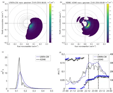
Wave data from the UWIN-CM are also compared to the available NDBC wave data in Fig. 4. Only data from NDBC buoy 42040 during the January high wind event are shown for wave model validation, as there were no wave data col-lected from buoy BURL1, and buoy 42040 stopped function-ing before the February event. Comparison of model output and observational data shows that the significant wave height is modeled accurately, especially under high winds, while the wave period could be slightly underestimated by the wave model. Mean wave direction is initially offset by∼30◦at the beginning of the high wind analysis period, but comes into good agreement about halfway through the analysis window. Wave data from buoy 42012 also showed good agreement with the UWIN-CM data near the buoy coordinates during the March event, but as drifters move further offshore dur-ing the high wind event, the nearshore location of the buoy becomes less representative of the conditions influencing the drifters.
J. Lodise et al.: Vertical structure of ocean surface currents 1633
Figure 2.Potential density(a), salinity(b)and temperature(c)data along the eastward-traveling transect shown in Fig. 1, measured by moving vessel profiler (MVP) conductivity–temperature–depth (CTD) casts taken on 28 January from 16:48 to 21:00 UTC.
NDBC. Figure 5c shows the 1-D wave density spectrum of the modeled and observed waves over the same hour dis-played in Fig. 5a, b. For validation of the Stokes velocity used by UWIN-CM, Eq. (2) is used to calculate the Stokes velocity using the 2-D wave spectrum from buoy 42040. Buoy 42040 is a 2.1 m diameter, Self-Contained Ocean Ob-servations Payload (SCOOP)-type buoy that extends down ∼1.68 m from the water line and reports wave spectrum data from 0.02 to 0.48 Hz (Bouchard et al., 2018). In order to make a fair comparison, we calculate the Stokes velocity us-ing the 2-D modeled wave spectrum from 0.0313 to 0.5 Hz, which are the closest corresponding frequency bins to that of the NDBC data. We then integrate the modeled Stokes ve-locity from the surface down to 1.68 m in order to accurately compare the buoy and wave model calculated Stokes
veloci-ties. Both the Stokes drift magnitude and direction calculated from the modeled and buoy wave spectrums are plotted in Fig. 5d.
Figure 3.Wind velocity magnitudes(a, b, c)and directions(d, e, f)during the hours preceding, and including, each high wind event. Dashed vertical black lines show the beginning and end of the high wind analysis periods. Dashed (solid) red lines indicate beginning of the hour over which the pre-existing regional circulation was estimated with undrogued (drogued) drifters.U10wind data from the UWIN-CM are plotted at the nearest point to every drifter location. Wind observations from NDBC buoys BURL1, 42040 and 42012 are plotted as well. Solid lines show sustained winds, while dashed lines show wind gusts. All wind directions are plotted as the direction in which the wind is traveling. Buoy 42040 was only operational during the first wind event and BURL1 did not record any wind direction data during the experiment.
motions from higher frequency waves under intense winds and coinciding strong surface currents, causing some dis-crepancy. The model- and buoy-calculated Stokes velocities do show good agreement with regards to direction.
3.2 LAVA and pre-existing regional circulation
Initial inspection of the total drifter velocities during each high wind event showed larger-than-expected spatial varia-tion in drifter velocities, including velocities which depict surface currents traveling to the left of the wind, which challenges previous wind-driven surface current theory and observations. Previous work that has studied instantaneous wind-driven dynamics over a range of spatial scales has il-lustrated the need to account for the circulation present be-fore the observed increase in synoptic winds in order to iso-late the wind-driven component of the flow (Sentchev et al., 2017; Berta et al., 2018). Based on these studies, we
hypothe-size that the spatial variability observed in the total velocities is due to the regional circulation that pre-existed the period of increasing winds, which retains its structure on timescales long enough to influence the surface flow during each high wind event.
tem-J. Lodise et al.: Vertical structure of ocean surface currents 1635
Figure 4.Significant wave height(a), mean wavelength(b), mean wave period(c)and mean wave direction(d)from the UWIN-CM and NDBC buoy 42040 during the January high wind event. Dashed vertical black lines show the beginning and end of the high wind analysis periods. Dashed (solid) red lines indicate beginning of the hour over which the pre-existing regional circulation was estimated with undrogued (drogued) drifters. Wave data from the UWIN-CM, plotted at the nearest point to every drifter location, are shown in blue. The solid black lines show the UWIN-CM output data closest to the coordinates of buoy 42040, while observations from buoy 42040 are shown with black dots. Wavelength data were not collected by this NDBC station.
poral scales on the order of 10 km and hours, respectively (Taillandier et al., 2006; Berta et al., 2015). LAVA has been used in previous studies to create velocity fields using purely Lagrangian data, as well as blending drifter trajectory data with Eulerian velocity fields derived from altimetry and HF radars. LAVA has proven especially useful when providing near-real-time (NRT) information that can be useful to first responders of oil spills, search-and-rescue efforts and other surface transport problems (Taillandier et al., 2006; Chang et al., 2011; Berta et al., 2014, 2015).
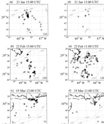
Given our hypothesis that, during the high wind events, the total velocity of the drifters is partly composed of the re-gional circulation that pre-existed the onset of high winds, an estimate for this circulation must be removed from the to-tal velocity of the drifters in order to isolate the wind- and wave-driven components. We utilize LAVA and the available drogued and undrogued drifter data in the region to create semi-instantaneous hourly Eulerian velocity fields for both drifter types, separately. The drifters used for the velocity field construction for each event are plotted in Fig. 6. The event on 22 January occurred very close to the initial time of deployment, while the drogued drifters were still tightly packed spatially and little drogue loss has occurred, leaving a
smaller, but adequate, number of undrogued drifters to utilize for the estimate of the pre-existing circulation. The events on 24 February and 20 March occur at a later time after deploy-ment, thus resulting in a more even amount of drogued and undrogued drifters that are also more evenly spread through-out the region; however, drogued drifters do show a tendency to converge upon one another, which is evident in the spatial organization of the drifters seen in Fig. 6.
Figure 5.2-D wave energy spectrum from(a)UWIN-CM and(b) NDBC buoy 42040 on 23 January at 00:00 UTC. Circles around the center of the plots show wavelengths ranging from 100 m (smallest) to 20 m (largest) on 10 m intervals.(c)1-D wave density spectrum from UWIN-CM and NDBC from the same hour.(d)Time series of Stokes drift velocity magnitude (solid lines) and direction (asterisks) calculated from the 2-D wave spectrum from buoy 42040 and the UWIN-CM model using Eq. (2). Vertical black lines indicate the period of velocity deconstruction. The UWIN-CM Stokes drift velocity plotted here is integrated from the surface down to 1.68 m, which is roughly the depth of the SCOOP-style NDBC buoy used at station 42040. All data from UWIN-CM are extracted from the nearest point to the location of buoy 42040.
Ta, is the larger time window over which consecutive velocity fields created using LAVA are averaged and should be shorter than the Lagrangian timescale (Taillandier et al., 2006). La-grangian timescales within this region have been calculated to be as small as ∼1–3 h, which corresponded to spatial scales ranging from 0.4 to 3.5 km (Gonçalves et al., 2019), and as large as∼1–3 d, corresponding to spatial scales rang-ing from∼10 to 35 km (Ohlmann and Niiler, 2005). Here,Ta is set to 1 h, which is adequately short given our assignment of 10 km as the typical horizontal length scale being resolved by LAVA.1x is the spatial resolution of the discretized ve-locity field and needs to be assigned such that1x < R, de-fined here as 1x=1.5 km (Taillandier et al., 2006; Berta et al., 2015). Drifter trajectories within 21x of one another are averaged to become single-drifter trajectories positioned along their center of mass before the production of Eulerian velocity fields (Berta et al., 2015).
After the Eulerian velocity fields are created, a kinetic en-ergy mask is also implemented to exclude small velocities
that are an artifact of assigning radially decreasing veloci-ties away from drifter locations using LAVA. To avoid these unrealistically small velocities, any values in the Eulerian ve-locity fields that represent less than 10 % of the hourly aver-aged kinetic energy in the velocity field are discarded. This relatively low threshold of kinetic energy was chosen to max-imize the coverage between the Eulerian velocity field esti-mates of the pre-existing regional circulation and drifter tra-jectory data during each high wind event.
J. Lodise et al.: Vertical structure of ocean surface currents 1637
Figure 6.Drogued(a, b, c)and undrogued(d, e, f)drifters used to create Eulerian velocity fields of the pre-wind-event regional circulation estimates using LAVA. Raw drifter locations are plotted at the end of the hour over which the velocity fields are created. Numbers in the bottom right corner of plots display the number of drifters used for each velocity field construction. Panels correspond to subdomains shown in Fig. 1.
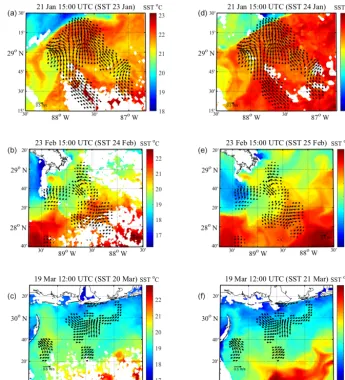
overlies the drifter trajectories during the high wind event. The Eulerian velocity fields used for analysis are plotted in Figs. 7 and 8. Each hour over which these velocity fields are created is also indicated in Fig. 3. The Eulerian veloc-ity fields are plotted on top of Aviso-derived 24 h averages of SST temperature, in order to validate the flow structures that are seen in the reconstructed velocity fields using LAVA. For each high wind event, the drogued and undrogued veloc-ity fields are directly compared to two SST fields: one cor-responding as closely as possible in time to the high wind event and one corresponding to the following day, in order to visualize the change in the pre-existing regional circulation during each high wind event (Figs. 7, 8).
Stokes drift estimates from the UWIN-CM during the time periods shown in Figs. 7 and 8, are on average an order
Figure 7.Eulerian velocity fields of the regional circulation that preceded each high wind event, created using LAVA for drogued drifters in the area. Also plotted are 24 h averages of Aviso SST data during(a, b, c)and after(d, e, f)each high wind event. Titles of each plot list the beginning of each hour over which the velocity field was created from drifter trajectories and the day corresponding to the Aviso SST data. The 24 h averages, produced by Aviso, are centered on 00:00 UTC of the day listed. In each velocity field, every third vector is plotted for visibility. Velocity fields on the left and right side panels are identical.
To provide a comparison to the LAVA-derived velocity fields, geostrophic velocity fields from altimetry data and NCOM velocities fields during each high wind event are shown in Fig. 9, plotted on top of associated SST temperature data. During the January and February wind events, we select the NCOM ocean velocity at 60 m depth at the beginning of the high wind analysis periods shown in Fig. 3. This depth is chosen based on the stratification shown in Fig. 2, with 60 m being just above the sharp pycnocline seen at∼80 m, thus being able to capture the mixed layer dynamics driving the regional flow at the surface, but deep enough as to not be affected by any wind stress in the model. As for the March event, much of the domain is bathymetrically limited due to its proximity to the coast, forcing the authors to use a shal-lower depth of 15 m for comparison. Velocity fields during,
rather than before, each high wind event are used to allow the model to account for any structural changes the flow may have experienced during the time gap between the LAVA-derived velocity fields and the analysis period during high winds. Such evolution of the regional circulation will not be observed by the geostrophic velocities from altimeter data as spatial and temporal resolution is much coarser.
3.3 Deconstruction of total surface current
The total drifter velocities, u¯T, calculated between each 15 min drifter position during the high wind events, are stored at the later drifter coordinate used for each calcula-tion. The time gap between the observation of the regional circulation,urc, and the beginning of the high wind
J. Lodise et al.: Vertical structure of ocean surface currents 1639
Figure 8.Eulerian velocity fields of the regional circulation that preceded each high wind event, created using LAVA for undrogued drifters in the area, plotted on top of the same 24 h averages of SST data shown in Fig. 7. Titles and data are plotted in the same manner as in Fig. 7.
a noticeable change in all the drifter trajectories across the given domain. Investigation of wind-driven currents at high temporal resolution has shown that the surface current re-sponse time to changing winds can be described as quasi-instantaneous, with the surface currents lagging the wind by ∼40 min (Sentchev et al., 2017). Having a temporal gap between these observations ensures the surface velocities, across the region, have ample time to adjust to the increas-ing winds before any calculations are made. In some cases, the time gap is extended to allow drifters to enter the re-gion where the corresponding observation of the pre-existing regional circulation exists. In addition, we stop the analy-sis for each high wind event at the apex of the increasing wind velocity magnitude, beyond which the drifters exhibit large inertial motions due to the decrease in momentum in-put from the wind. The drifter trajectories, during the period
over which the deconstruction of the total drifter velocities is performed, are shown in Fig. 10.
From the full drifter velocities, calculated on 15 min inter-vals during each wind event, we subtract the nearest point ve-locity in the estimated LAVA veve-locity field of the pre-existing regional circulation,urc. Each velocity field has a spatial
Figure 9.Aviso-based geostrophic velocities(a, b, c)and NCOM velocities(d, e, f)associated with each high wind event, along with relevant SST data. SST maps were chosen based on coinciding timing with each high wind event and/or visibility of circulation patterns. The date of each daily geostrophic velocity or 3 h NCOM velocity field are listed for each panel. Dates of SST data are listed in the same manner as in Figs. 7 and 8. NCOM velocities are plotted at 60 m depth for the January and February events, while they are plotted at 15 m for the March event. Velocity arrows for geostrophic velocities are scaled twice as large as those of NCOM fields.
same manner. For accurate comparison, any data points along the drifter trajectories that were excluded during the subtrac-tion of the LAVA velocity field estimates were also excluded from the calculation involving the Aviso and NCOM velocity fields.
The subtraction of multiple hourly adjacent LAVA veloc-ity fields, earlier and later in time, were examined a pos-teriori for each event and found to produce similar end re-sults. The hourly LAVA velocity fields chosen for this analy-sis were those that had the most data points in common with the respective drifter trajectories during the high wind event or those that retained a similar amount of data points dur-ing the subtraction (within 3.5 % of the maximum amount of
J. Lodise et al.: Vertical structure of ocean surface currents 1641
Figure 10.Drogued(a, b, c)and undrogued(d, e, f)drifter trajectories during the hours of analysis for each high wind event. Time periods over which the total velocity deconstructions were calculated are shown in each title. Portions of the trajectories shown in black (red) depict segments which overlap (do not overlap) spatially with each respective LAVA-derived Eulerian velocity field in Figs. 7 and 8. Trajectories missing head markers are a result of either drogue loss or lost GPS transmission during the experiment. The total number of retained trajectory data points, defined as number of drifter days given 15 min time steps, and the percentage of coverage between trajectories and each respective Eulerian velocity field in Figs. 7 and 8 are listed within each plot.
After subtracting the estimates for the pexisting re-gional circulation from the full drifter velocities during the high wind events, the remaining velocity is an estimate for the combined wind- and wave-driven flow (us+uw), referred
to here after as the wind-wave-driven velocity. To further de-construct this velocity estimate, we subtract the UWIN-CM-modeled Stokes drift velocity (us) fields, again at the nearest
point to each drifter location for each 15 min interval. Be-cause the large wind-driven events being analyzed are of syn-optic scale, the UWIN-CM-modeled Stokes velocity andU10 winds are relatively uniform in the region of study, making the 4 km resolution of the data adequate to perform meaning-ful calculations in this manner.
Because the drogued drifters display a filtering charac-teristic of the surface Stokes drift, as illustrated in labora-tory testing performed by Novelli et al. (2017), the Stokes drift at 0.4 m depth is used for the calculation with drogued drifter-derived velocities (0.4 m being the vertical center of the drogue). From the undrogued-drifter-associated veloci-ties, we subtract the surface (z=0 m) Stokes drift velocity. After subtracting the wave-driven component,us, from the
wind-wave-driven velocity, we are left with an estimate for the average wind-driven drifter velocities,uw, over each
mod-Figure 11.Scatter plots of deflection angles of drogued(a, c, e)and undrogued(b, d, f)drifter velocities before(a, b)and after(c, d, e, f) sub-tracting estimates for the regional circulation during the high wind periods analyzed. Panels(c)and(d)are created using the NCOM velocity fields during the high wind events (Fig. 9), while panels(e)and(f)use the LAVA-derived estimates observed before each high wind event (Figs. 7 and 8). Data points that do not have both individual drifter velocity measurements and coinciding data in the LAVA-derived Eulerian velocity fields of the pre-existing circulation during the high wind event are not included in any panel. Deflection angles are plotted against theU10wind magnitude from the UWIN-CM model at the nearest point to the drifter locations in the domain.
eledU10wind data, using theU10wind velocity datum at the nearest point to each drifter location at every time step.
4 Results
The main flow features seen in the estimated Eulerian veloc-ity fields and SST fields show evidence of flow features hav-ing spatial scales on the order of tens of kilometers (Figs. 7 and 8). Observations of smaller flow features in the velocity fields are limited by the 1.5 km resolution and typical length scale of 10 km set by the chosen LAVA configuration. The regional circulation observed, by either drifter type, prior to the wind events on 24 February and 20 March shows an abun-dance of meanders, eddies and frontal features, whereas the regional circulation pre-existing the wind event on 22
J. Lodise et al.: Vertical structure of ocean surface currents 1643
Figure 12.Average of the Eulerian LAVA-derived velocity field es-timates of the pre-wind event regional circulation plotted as a per-centage in time of the average combined wind- and wave-driven flow for drogued and undrogued drifters. Dashed vertical lines de-pict the analysis period for the total velocity deconstruction.
during the high wind event, the pre-existing circulation es-timates seem to be valid for an appreciable amount of time, evident in the overlap between eddies, fronts and filaments observed in the SST field and the velocity vectors created with LAVA 2–3 d previously.
Comparison between Figs. 7 and 8 with Fig. 9 displays ro-bust discrepancies between the velocity fields created using LAVA and drifter data, altimetry data and NCOM. The coarse resolution of the geostrophic velocities does not capture the circulation highlighted in the SST data. The geostrophic ve-locities are also appreciably smaller than either LAVA or NCOM (vectors for the geostrophic velocities in Fig. 9 are magnified by a factor of 2 compared to those of the NCOM circulation). Velocities showing the NCOM circulation seem to better complement the structures observed in the SST data compared to the geostrophic velocities (Fig. 9); however, compared to the LAVA-derived velocity fields in Figs. 7 and 8, there still exists a fair amount of disagreement between the NCOM and LAVA velocity fields, possibly the most pro-nounced example being the velocity fields associated with the January wind event.
The trajectories of both drogued and undrogued drifters during the hours of increasing winds, over which the total ve-locity deconstructions were performed, are shown in Fig. 10. Overall, the trajectories show that the larger-scale synoptic
Figure 13.Number of undrogued(a)and drogued(b)drifter posi-tions where the velocity deconstruction was performed, binned by wind velocity magnitude on 0.5 m s−1intervals. Point velocity mea-surements calculated from drifter trajectories that do not coincide spatially with available data in the pre-existing circulation velocity fields are not included.
winds and coinciding wave-induced motions are the domi-nant driving forces in the drifter movement, evident in the similarities in drifter tracts across each domain. Influence of the pre-existing regional circulation can also be observed in the variability among drifter trajectories. The undrogued trajectories seem to show less variability across the domain than for the drogued case, suggesting the wind- and wave-driven components are even more dominant in the surface layer measured by the undrogued drifters.
Figure 14. Average deflection angles at drifter locations during periods of high wind binned by UWIN-CM wind magnitudes on 0.5 m s−1 intervals. Horizontal dotted lines denote 0, 45 and 90◦ to the right of the wind. (a)UWIN-CM Stokes drift velocity di-rection at the surface (0 m) and at 0.4 m depth.(b)Velocity direc-tion of drogued and undrogued drifters after the subtracdirec-tion of the pre-existing circulation estimate.(c)Velocity direction of the purely wind-driven component of the drifter velocities. All error bars show
+/−1 standard deviation within each bin. Data in wind bins lower than 11.5 m s−1were omitted due to lack of data points and large standard deviations.
magnitude from the UWIN-CM model, closest to the drifter location at the time of the velocity measurement.
It is evident from Fig. 11 that the resulting scatter plots, after subtracting the LAVA-estimated velocities, have a more organized and compressed scatter than that of the total drifter velocity deflection angles. This is especially apparent for the drogued drifter case. The scatter plots created after the NCOM velocity fields have been subtracted from the full drifter velocity and have a wider, more disorganized spread than that of the full drifter velocities, with a large portion of the deflection angles being directed to the left of the wind direction for both drogued and undrogued drifters.
Result-Figure 15.Average velocity magnitudes at drifter locations dur-ing periods of high wind binned by UWIN-CM wind magnitude on 0.5 m s−1intervals.(a)UWIN-CM Stokes drift velocity magni-tude at the surface (0 m) and at 0.4 m depth.(b)Velocity magnitude of drogued and undrogued drifters after the subtraction of the pre-existing circulation estimate.(c)Velocity magnitude of the purely wind-driven component of the drifter velocities. All error bars show
+/− 1 standard deviation within each bin. Data bins omitted in Fig. 14 are also excluded.
J. Lodise et al.: Vertical structure of ocean surface currents 1645
The average velocity magnitudes of the calculated wind-wave-driven drifter velocities are compared to the average magnitude of the LAVA-derived pre-existing regional circu-lation for each wind event and drifter type in Fig. 12. The magnitude of the regional circulation is plotted as a percent-age of the combined wind- and wave-driven velocity mag-nitude. This percentage decreases as the wind- and wave-driven effects become increasingly large during each high wind event. During the analysis periods over which we de-construct the total surface current (shown by vertical lines in Fig. 12), the pre-existing circulation is 30 %–45 % as large as the combined wind-wave-driven velocity calculated using drogued drifters and 25 %–30 % as large as that measured by undrogued drifters.
The wind-wave-driven, wind-driven and wave-driven (Stokes drift) velocities are binned by wind magnitude on 0.5 m s−1intervals. The total number of drifter positions, per wind bin, where the drifter velocity deconstruction is per-formed, are plotted in Fig. 13, which shows that the most robust results exist over wind bins from 14.5 to 18 m s−1for both drogued and undrogued drifters. It should be noted that although the sample size varies considerably between drifter types and over the assigned wind bins, both drifter types have substantial sample sizes over most wind bins presented, given the relatively short time periods of analysis. The sam-ple size of drifter measurements is also listed for each high wind event in Fig. 10. Averages and standard deviations of the velocity components were computed within each bin. The average deflection angles from the wind direction of the Stokes velocity, wave-wind-driven velocity and wind-driven velocity for each respective drifter type are shown in Fig. 14. The magnitudes of the same velocity components are plotted as a percentage of the wind magnitude in Fig. 15. Figures 14c and 15c are obtained by subtracting the given Stokes drift ve-locity (Figs. 14a, 15a) from the estimated wind-wave-driven velocities (Figs. 14b, 15b). Bins lower than 11.5 m s−1have been omitted in Figs. 14 and 15 due to lack of data points and large variation of deflection angle in the given bins. Er-ror bars indicate 1 standard deviation about the mean for each bin (Figs. 14, 15).
The average wind-wave-driven component of the un-drogued drifter velocity varies with increasing wind speed, traveling between ∼4 and 40◦, to the right of the wind, as winds increase from 11.5 to 20 m s−1(Fig. 14b). On average, the magnitude of this velocity component varies from 4.5 % to 7.1 % of the wind speed (Fig. 15b). For the drogued drifter case, the deflection angle of the wind-wave-driven compo-nent varies from ∼26 to 60◦, as winds increase over the same range, traveling at 2.8 %–4.6 % of the wind speed, on average (Figs. 14b and 15b). The total wind-wadriven ve-locities exhibit larger deflection angles as wind speeds in-crease, with the drogued-drifter-derived velocity traveling at a slower speed and being deflected ∼5–28◦ further to the right than that of the undrogued drifters.
Our estimates for purely wind-driven velocity components (Figs. 14c and 15c) show the undrogued drifter wind-driven velocity traveling∼5◦to the right of the wind, at 6.0 % of the wind speed during 12 m s−1 winds. The deflection an-gle gradually increases to∼55◦to the right of the wind as wind speeds increase to 20 m s−1. The average velocity mag-nitude varies between 3.4 % and 6.0 % of the wind speed over this wind interval. The deflection angle of the drogued drifter wind-driven velocity ranges from ∼30 to 85◦, again with higher deflection angles occurring at higher wind speeds. The velocity magnitude of this component varies from 2.3 % to 4.1 % of the wind speed over the given wind speed interval. The difference in deflection angle between undrogued and drogued wind-driven velocities varies between∼8 and 30◦, with the drogued drifter component traveling further to the right at a slower velocity. In both cases, there seems to exist an increase in deflection angle with increasing wind speed.
5 Discussion
northern gulf where smaller-scale structures dominate. The increased scatter of the deflection angles, shown in Fig. 11c– d, also implies that the regional circulation is not accurately represented by the NCOM ocean velocities. The increased agreement of the structures seen in SST data and the LAVA-derived velocity fields, as well the comparison between scat-ter plots shown in Fig. 11, reveals that the velocity fields cre-ated using the observational drifter data are more equipped to described the regional circulation specific to this area than altimetry-based or modeled velocities.
Comparison of scatter plots in Fig. 11a, b and e, f indicates that the pre-existing regional circulation still influences the velocities measured by both drifter types during these large wind-driven events. The scatter of deflection angles between different drifter types also suggests that the relatively deeper layer measured by the drogued drifter exhibits larger vari-ation in velocity due to the regional circulvari-ation component of the flow. The velocities observed with undrogued drifters seem to be more dominantly driven by the wind and wave components, as removing the influence of the regional cir-culation results in a less drastic compression of the scatter. In both the drogued and undrogued cases, the removal of the LAVA-estimated regional circulation results in a decrease in the standard deviation of the deflection angle for all wind bins from 11.5 to 20 m s−1.
Comparison of the relative magnitudes of the combined wind-wave-driven velocities and the pre-existing circula-tion estimates confirms that the drifter velocities are domi-nantly wind- and wave-driven during the high wind periods (Fig. 12). Analysis of the plots in Fig. 12 led the authors a posteriori to determine the optimal windows for the veloc-ity deconstruction results during the high wind events. With respect to the subtraction of the pre-existing regional circula-tion and the improvement of the scatter in defleccircula-tion angles (seen in Fig. 11e, f), the most robust results, for both drifter types, occur when the relative strength of the wind-wave-driven flow to the pre-existing regional circulation reaches a plateau (Fig. 12). This is also when the wind, and therefore the wind-wave-driven component, is the strongest, which suggests that any error introduced during the velocity de-construction makes up a smaller percentage of the calcu-lated velocities. Extending the velocity deconstruction anal-ysis windows, by 2 h before and 2 h after, does not signifi-cantly change the averages and trends shown in Figs. 14 and 15 but does, however, slightly disorganize the scatter of the deflection angles seen in Fig. 11e, f. This investigation of sensitivity also aided in determining the optimal time peri-ods for analysis.
Figure 14b shows that the estimated deflection angle of the combined wind- and wave-driven velocities of drogued and undrogued drifters varies significantly with increasing wind velocity. Since the deflection angle of the Stokes drift velocity (Fig. 14a) is almost constant with wind speed, the increase in deflection angles seen in Fig. 14b is most likely due to a change in the wind-driven momentum input. The
increased deflection angle observed between the two drifter types seems to be predominately wind driven based on the relative magnitudes of Stokes drift and estimated wind-driven velocities (Fig. 15). Classical Ekman theory is based on the balance between Coriolis and vertical viscosity in the water column, which, given the parameterization for wind stress and viscosity assigned by Ekman (1905), results in a wind-driven surface current deflected 45◦to the right of the wind in the Northern Hemisphere, which spirals to the right and decreases in magnitude with depth. In contrast to Ekman, the “slab” solution, based on enhanced surface mixing due to breaking waves and shear-induced turbulence, prescribes a linear decrease of wind stress with depth, resulting in a sur-face current which travels 90◦ to the right of the wind uni-formly with depth (Pollard and Millard, 1970).
The findings presented here seem to support aspects of both the Ekman and slab solutions, as there does appear to be a rotation of the wind-driven drifter velocities with depth, but overall, these velocities display a larger deflection than predicted by Ekman at larger wind speeds. This can pos-sibly be explained by enhanced vertical mixing under high wind and wave conditions, which acts to diminish the effects of stratification and distribute wind-driven momentum into the water column. This theory motivates the assignment of a linearly decreasing wind stress with depth used in the slab model solution by Pollard (1970), which results in deflec-tion angles of 90◦ over all depths of the mixed layer. The observed increase in deflection angle with wind speed may suggest a gradual change in wind-driven flow regimes, from surface Ekman dynamics to more slab-like dynamics, as in-creasing wind velocity and subsequent turbulence from ver-tical shear and breaking waves mix momentum verver-tically in the wind-driven layer. However, there still exists a rotation of the wind-driven current with depth which cannot be ex-plained using slab-like dynamics alone.
influ-J. Lodise et al.: Vertical structure of ocean surface currents 1647
ence of large wind events lasting 1–3 d. After subtracting the geostrophic component of the flow to isolate the wind-driven current, they found surface velocity deflection angles and magnitudes of 25–30◦and∼2 % of the wind speed, re-spectively. More details of these previous studies on wind-driven dynamics can be found in Table 1.
The findings portrayed in this paper seem to be within the range of previously reported results for wind-driven sur-face flows with discrepancies likely resulting from the differ-ences in the depth of the measurement, range of wind magni-tudes, upper ocean stratification or methodology in isolating the wind-driven component. Several of these previous studies also utilized datasets with a portion of surface current mea-surements occurring close to the coast, where topography could have added noise to the measurements (Poulain et al., 2009; Kim et al., 2010; Röhrs and Christensen, 2015; Berta et al., 2018). With the exception of Ardhuin et al. (2009), these past studies have not accounted for Stokes drift in their measurements, sometimes due to negligible wave influence under low wind conditions, possibly resulting in smaller de-flection angles due to the near alignment of winds and wave direction (Poulain et al., 2009; Kim et al., 2010; Röhrs and Christensen 2015; Sentchev et al., 2017; Berta et al., 2018). The UWIN-CM-modeled Stokes velocity used for this study seems to be in good agreement with the full Stokes veloc-ity magnitude and deflection angle, with respect to the wind, presented by the previous literature (Ardhuin et al., 2009).
We explore the possible influence of wind-driven effects during the observation of the pre-existing regional circula-tion by conducting a sensitivity test where an estimated wind-driven velocity (based on the UWIN-CM wind velocities) is removed from the LAVA-derived velocity fields before the total velocity deconstruction is performed. Relying on previ-ous literature, we estimate that during low wind conditions, the undrogued drifters travel at 3.5 % of the wind, being de-flected 5◦ to the right, while the drogued drifters travel at 1.5 % of the wind, being deflected 25◦ to the right. These values were chosen, based on the results of all the literature shown in Table 1, to represent moderate wind-driven effects on the surface drifters. Laboratory testing and field exper-iment results using the CARTHE drifters also aided in as-signing the differential velocities between drifter type (Lax-ague et al., 2018; Novelli et al., 2017). Performing the total velocity deconstruction with this estimated wind-driven ef-fect removed from the pre-existing circulation, on average, results in a decrease of wind-driven velocities magnitudes by 0.58 % and 0.34 % of the wind velocity for undrogued and drogued drifters, respectively. The average deflection angles of the wind-driven component of both drifter types become more aligned with the wind by about 5◦for drogued drifters and 7◦for undrogued. While there is some change in the fi-nal magnitudes and deflection angles calculated, the overall trends seen in Figs. 14 and 15 do not change as a result of this sensitivity analysis. Additionally, the scatter plots of deflec-tion angles (Fig. 11e, f) become slightly more scattered
(stan-dard deviation slightly increased) with this estimated wind influence removed and become even less organized when the estimated wind-driven velocities during the low wind periods are increased further. Because the true values of the wind-driven velocity components during these low wind-periods are not well known, and the standard deviations of deflec-tion angle are slightly increased by accounting for such, we do not account for any wind-driven influence during the low wind periods for the final results. The assignment of decreas-ing velocities away from the drifter locations up to a length
R, prescribed by the LAVA algorithm, in addition to aver-aging, acts to smooth out the absolute velocities of the in-dividual drifters, which adds complexity to accounting for wind-driven effects during these low wind periods.
Another source of error in the wind-driven measurements reported here is the possible evolution of the regional circula-tion during the time gap between the observacircula-tion of the pre-existing regional circulation and the velocity deconstruction during the high wind period. Although difficult to quantify given the available data, the regional circulation is evolving, to a certain extent, during the time gap between the obser-vation of the regional circulation and the analysis periods of high winds. In addition, the regional circulation could begin to be modified through interactions with the large wind- and wave-induced currents. The extent to which this is occurring can be seen qualitatively in Figs. 7 and 8 by comparing the change of the SST fields in time. One example of this is ev-ident in the southeastward progression of the front seen in the SST fields associated with the January high wind event. The movement of this front seems to generally mimic the movement of the drifters during this high wind event shown in the top panels of Fig. 10. The overall timescales on which these flow features evolve or are altered by each high wind event are beyond the scope of this paper, given the available dataset. However, the relatively short timescales of these pe-riods of high winds and the overall agreement between the pre-existing circulation estimates and the SST fields (shown in Figs. 7 and 8) suggest that the method of velocity decon-struction used here is adequate. In addition, the decreased variability seen in the deflection angles after the subtraction of the pre-existing regional circulation (Fig. 11) suggests, a posteriori, that the regional circulation does maintain its structure to a reasonable extent during the periods of increas-ing winds beincreas-ing analyzed.
com-bined wind-wave-driven velocity magnitudes of drogued and undrogued drifters (∼2 % of the wind speed on average) in the current study are in good agreement to that of laboratory studies using half-scale drifters and a past field experiment using full-size drifters (Laxague et al., 2018; Novelli et al., 2017). As mentioned above, laboratory testing of undrogued drifters showed that the total velocity slip could be as high as 14 cm s−1 but was shown to decrease to only 1 cm s−1 with increasing wind speeds (over a range of 15–23 m s−1 in the lab) due to the sheltering of drifters from the wind by increasing wave heights (Novelli et al., 2017). This could partly explain the gradual decrease in wind-driven velocities for both drifter types from wind bins 11.5–18 m s−1, espe-cially given the relatively high wind-driven velocities seen at lower wind bins. Exactly how much wind slip is occur-ring duoccur-ring specific wind velocities and wave heights in the real ocean is difficult to determine, but the average magni-tude of the observed vertical shear seems to be in relatively good agreement with past experiments and laboratory testing performed with these drifters (Laxague et al., 2018; Novelli et al., 2017).
The momentum input from large breaking waves into the surface currents at the very high wind speeds studied here could also cause an increase in velocities observed in the wind-driven surface currents estimated from either drifter type. In addition, the surfing behavior of the undrogued drifters could amplify this increase in observed velocities further. Velocity slip due to wind and breaking waves could also account for some of difference seen in deflection an-gles between the drifter types, as the influence of wind and waves would keep the undrogued drifters more in line with the wind. Ardhuin et al. (2009) attributes larger deflection angles of wind-driven currents to enhanced mixing due to wave breaking, which could be a congruous theory to our observation of increasing deflection angles at higher wind speeds. Enhanced mixing caused by breaking waves acts to mix the vertical momentum of surface currents, likely result-ing in larger deflection angles at shallower depths (Rascle et al., 2006).
The results presented here, to the authors’ knowledge, are among the few studies able to reported estimates of the ver-tical shear of wind- and wave-driven velocity components in the upper 1 m of the ocean under this regime of high winds (11.5–20 m s−1). The combined wind-wave-driven velocity of the undrogued drifters calculated here is, on average, ∼1.6 times greater than that measured by drogued drifters for the wind magnitudes presented. These results support the finding of Laxague et al. (2018), which showed that, in the presence of negligible stratification in the upper layer, total surface currents in the upper 1 cm are twice as fast as the average current over the first 1 m (measured to be 0.57 and 0.3 m s−1, respectively) due to wind- and wave-driven verti-cal velocity shear. It should also be noted, however, that ver-tical shear in the presence of strong mixing (i.e. wave break-ing) acts to diminish vertical velocity gradients, which could
suggest some of the shear observed is due to the velocity slip of the undrogued drifters (Sutherland et al., 2016). The true novelty of the results presented here lies in the instantaneous estimates for the vertical shear of the purely wind-driven velocities calculated from each drifter type made possible through the method of velocity deconstruction used here. The deconstruction of the total velocity measured from drogued and undrogued drifters gives us an estimate, directly related to the wind velocity, of the wind-driven vertical shear at the very surface of the ocean, which has proved difficult to mea-sure by previous studies and has significant implications for surface transport problems in the real ocean.
The high wind events focused on here only occurred for a small number of days during the LASER campaign, which is typical for the northern Gulf of Mexico in the winter. Since the velocity profile within the upper meter has been shown to be very dynamic, being affected by the general oceanic circulation as well as local wind-wave-driven mechanisms, it is important to observe near-surface currents under differ-ent environmdiffer-ental conditions and at greater vertical resolu-tion. Attention also needs to be given to the transport of La-grangian particles by breaking waves which induce vertical motion and mixing which can alter wind-driven currents.
6 Conclusions
We use a combination of stored output data from the UWIN-CM fully coupled atmosphere–wave–ocean model and ob-servational trajectory data from both drogued and undrogued CARTHE drifters to calculate an estimate for purely wind-driven drifter velocities during periods of strong, increasing winds. The use of colocated drogued and undrogued drifters provides measurements for the vertical shear between the upper 5 cm and upper 60 cm surface layers. Using LAVA, we are able to create velocity fields in the hours leading up to the high wind events studied that serve as an esti-mate for the pre-existing regional circulation which is found to still affect the drifter velocities during periods of high winds. After subtracting the regional circulation from our measured drifter velocities, we analyze the relationship be-tween wind velocity, Stokes drift and wind-driven velocity of each drifter type. On average, we find the wind-driven ve-locity component between drifter types to decrease in mag-nitude and rotate to the right of the wind with depth, with the undrogued (drogued) component traveling∼5–55◦ (∼30– 85◦) at 3.4 %–6.0 % (2.3 %–4.1 %) of the wind speed over the range of 12–20 m s−1. Both wind-driven velocities display an increase in deflection angle with increasing wind speed, sus-taining an average difference of 8–30◦ between the layers sampled.