The Problem of Optimal Delivery Sizes in the
Logistics System of a Manufacturing Enterprise
Dariusz Milewski
Faculty of Management and Economics of Services University of Szczecin
Cukrowa Street 8 71-004 Szczecin, Poland, [email protected]
ABSTRACT
When determining the optimal size of the deliveries of a product to a warehouse, one should consider not just a single factor such as warehousing or the cost of keeping inventory, but also other factors such as the cost of ordering or transportation. The factors to be considered in such a decision become more complex when the situation involves several products or an entire distribution system that might consist, for example, of one or more central warehouses, as well as regional or local warehouses or distribution centers. This paper addresses the problem of optimizing logistics decisions in a two–level inventory management system, taking into consideration also the transportation costs involved. Using a Polish chemical manufacturing company as the case study, the author developed a model of total costs for the distribution network and, for simulation purposes, applied a computer program as a virtual model of the production company and its logistics system. The model is very detailed because it reproduces logistics processes on daily basis.
International Journal of Business and Information
1.
INTRODUCTION
Optimizing a logistics decision is not an easy task when a number of factors are taken into consideration. The task becomes even more difficult when the relationship between a certain decision and its effectiveness has a non-linear character. In such a case, it is hard to find a proper mathematical function to reflect this relationship. Using mathematical formulas as optimization tools can lead to incorrect solutions (not optimal) if the formulas do not consider these relationships. Even very simple optimization tasks, such as determining the optimal size of the delivery of one product to one warehouse, can require the use of a relatively complex model to ascertain optimal solutions. One reason for the complexity is the need to incorporate transportation costs. The complexity increases when solutions are sought for a wide range of products in the distribution network.
The economic order quantity (EOQ) formula is well known and widely described in the literature (not only in the field of logistics). In its basic form, the formula is a mathematical model that includes only two costs: inventory holding costs and ordering costs. There are also modified forms of EOQ, some of which also take into account changes in purchase costs, which vary when a supplier offers a quantity discount.
The limitations of the EOQ formula have also been identified. The main disadvantage of the formula is the assumption that use of the goods that are stored will remain stable. Another disadvantage is the linear character of process relationships, which rarely occurs in the real world. The formula uses the costs of placing orders, which are supposed to be fixed. Transportation costs can be used in the formula if the same kind of transportation mean is used (of the same loading capacity, but with different capacity use). A problem occurs, however, when the transportation mean is changed because, in such case, the relationship between quantities and costs becomes non-linear.
The level of difficulty increases when several levels of warehousing are taken into consideration. This situation occurs most frequently, for example, in companies selling consumer goods. In optimizing processes of physical distribution, one must consider transportation costs when goods are moved within a company’s own distribution system; for example, from the factory to the
company’s own centers. (In the supply of materials for production, or in case of
transportation; therefore, transportation costs are not considered in receiver calculations, unless they affect profitability.) So, there is a trade-off between transportation and inventory and warehousing costs when decisions concerning deliveries are made. One must also consider the levels of the system. Solutions that are beneficial for local or regional distribution centers can be disadvantageous for a central warehouse or a factory that supplies these centers.
The primary goal of this paper is to examine problems relating to the optimization of decisions about complex logistics processes. The supplementary goal is to prove that it is very important that the practical aspects of business processes be reflected in theoretical mathematical models.
The paper contains five sections. Section 2 is a literature review of inventory management models in simple and complex systems. Section 3 presents basic information about the Polish chemical manufacturer used in the current research as a case study. Section 4 describes the problem of considering transportation costs in mathematical optimization models. Section 5 focuses on the problem of finding the optimal order quantity to be sent by distribution centers in a more complex system – namely, the distribution system of a
manufacturing company. Section 5 also presents simulation models in both mathematical and electronic forms and discusses how they were used in this study to calculate different distribution strategies. Section 6 presents the study conclusions and offers recommendations for modeling in logistics.
2.
REVIEW OF THE LITERATURE
A number of research studies focus on the optimal parameters of the replenishment process (e.g., quantity of deliveries to a warehouse, reorder point, level of customer service). The classical method for finding the optimal lot size of a delivery is to use the economic order quantity (EOQ) formula. The formula, however, includes only the trade-off between inventory carrying cost and setup or ordering cost. It also requires conditions that are difficult to meet in many practical situations. Quite often, other factors (such as transportation costs) must be taken into consideration.
International Journal of Business and Information distribution systems where inventory and transportation costs are taken into account. Some authors criticize the approach, however, and note that transportation unit costs are not fixed, but change along with the change in order quantity [Zhao, Wang, Lai, and Xia, 2004].
The simplest way to solve the problem is to add transportation costs to the total purchasing costs that correspond to an EOQ [Coyle, Bardi, and Langley, 2003; Buffa and Reynold, 1977], and then to compare the different levels of costs and choose the minimal one. Another method, based on a similar rule, is to calculate an EOQ for each class of freight rates. This approach is the most accurate but also the most labor-intensive way to find an optimal solution. Even with the use of computer technology, it is not easy to find optimal solutions when a company purchases hundreds or thousands of commodities. A model could be useful, therefore, even if it is not the most precise, so long as it allows one to determine transportation costs in a simpler way.
Langley [1980] compared four models with different transportation costs functions: constant, proportional, exponential, and inverse. Two of the models (exponential and inverse) are quite similar to the real curve of the rates. The inverse model is the most accurate, but it is hard to use in the EOQ formula. Langley [1980] also considered the problem of incorporating the functional relationship between transportation and inventory management and the necessity of creating a model for decision-making purposes. Swenseth and Godfrey [1996] developed models with five different alternatives of functions – proportional, adjusted inverse, constant, exponential, and inverse – and analyzed the adjustment of these functions to the real rates. But, again, although these models can be used for simulation of transportation costs, they are very difficult to incorporate into the EOQ formula. All of these models reflect one interesting relationship: the more complex the model, the better its adjustment to real conditions; but, the simpler the model, the greater the possibility of using it in an optimization formula.
The preceding models refer to simple optimization in which one product in one place is considered. There is a need, however, for decision-making tools that can be used for optimization of entire logistics systems. An integrated model for joint inventory replenishment was proposed by Mutlu and Çetinkaya [2010] with regard to consolidation of shipments. Models with distribution-production relationships can be found in Prasad and Sankaran [1996] and likewise in Cordeau, Pasin, and Salomon [2003], and Fokkens and Puylaert [1981]. These authors generally used aggregated data and a category of unit costs that is fixed. Recently, the problem of optimizing costs in distribution systems was addressed by Madadi, Kurz, and Ashayeri [2010], who proposed two models that consider variable transportation costs. These models are also aggregated, and refer to the problem of choosing between centralized and decentralized distribution systems. Even if a model relates to the complexity of the relationship between the size of a delivery and logistics costs, it is used, in many cases, as a simulation model rather than as an optimization model in the strictest sense. This situation illustrates that it is not easy to build an optimization tool that enables one to easily find optimal solutions. This difficulty is addressed in the works of Langley [1980], Swenseth and Godfrey [1996], Meyer, Peck, Stenason, and Zwick [1959], Constable and Whybark [1978], Das [1974], Ferguson and Glorfeld [1981], Stenger, Coyle, and Price [1977], and Saker, Maulloo, and Rahman [2004].
The aim of building models like the one presented in this paper is to determine the relationships among logistics processes in complex logistic systems and to ascertain how these relationships affect the effectiveness of the system.
3.
APPLICATION OF THE EOQ FORMULA: A CASE STUDY
For the case study in this paper, the author chose the company Zakłady
Chemiczne Police, S.A., which is a Polish producer of chemical products. The company, which is located in northwest Poland, produces, among other things, fertilizers for agriculture, which are sold under registered brand names:
POLIWAP®
POLIDAP®
POLIFOSKA®
POLIMAG®
International Journal of Business and Information In all, the company produces 12 assortments of fertilizer. The products are distributed through its factory warehouse and six regional distribution centers (Figure 1). The yearly sales to all customers total 1.5 million (mln) tons. The yearly sales in one center total D = 40,000 tons. The rest is sent directly to customers by sea, rail, and road transportation. The sales are seasonal (Table 1).
Figure 1. Location of Distribution Centers of ZCh Police, S.A.
Source: Website www.zchpolice.pl
Table 1
Seasonality of Fertilizer Sales by ZCh Police
Month Share
January 6% February 10% March 15% April 15% May 3% June 3% July 3% August 7% September 15% October 15% November 4% December 4%
The following discussion explains how mathematical formulas could help in finding the optimal size of a delivery to a distribution center and a reorder point for ZCh Police, S.A. One of the company’s six distribution centers will be treated as an independent selling point and not as an element of the distribution system, which means that the optimization criterion is the minimum total costs of replenishment.
The data used for calculations are as follows: D – yearly demand – 40 000 tons
d
– average daily demand of one product in one center – 13 tonsd
– standard deviation of daily demand of one product – 4 tons L – lead time – 3 days (assuming all deliveries will be on time) LCS – logistic customer service – 99% (99% of goods are in stock) sp– average selling price of products – 1,270 PLN per tonp– costs of production (treated as value of product) – 600 PLN per ton
o
c
– ordering costs per one order – 50 PLNi
c
– annual carrying costs of inventories – 10%1w
c
– the costs of warehousing – 30 PLN/per 1 ton per year (0,12 per ton daily)The classical mathematical formula for economic order quantity (EOQ) is:
p
c
c
D
EOQ
i o
2
1 These costs (interest on investment of working capital, deterioration, and shrinkage of
International Journal of Business and Information But, if warehousing costs are included, the formula is modified:
p
c
c
c
D
EOQ
i w
o
2
Reorder point (ROP) for replenishment:
L
z
L
d
ROP
dInteger “z” for 99% customer service is 2.30 (taken from tables).
Use of the above formulas produces these results: EOQ = 196 tons
ROP = 675 tons
These figures mean that deliveries have to be made daily (daily sales are 157 tons), which is an impossible feat because the lead time is 3 days. The calculated ROP indicates that the EOQ should be higher. This example proves that, in looking for optimal replenishment parameters when the demand is variable, one must consider order sizes and reorder points together. In other words, there is a relationship between delivery quantities and safety stocks. In addition, there is also the problem of optimal safety stock and optimal level of customer service (trade-off between inventory costs and costs of lost sales). The problems relating to relationships between cycle and safety stocks and other relationships in complex systems were described by the author of this paper in several publications [Milewski, 2006, 2007, 2009].
The optimization problems become more complicated than depicted in the EOQ model. It seems that a better method might be simulation. This problem is addressed later in this paper.
equipment). It may happen that, in order to avoid the waiting costs of transportation, a company may increase the loading potential, which would change not only the amount of the costs, but also the structure of these costs. This situation is also difficult to consider in a mathematical model.
4.
FREIGHT COSTS IN ROAD TRANSPORT:
THEORETICAL PROBLEM AND PRACTICAL ASPECTS
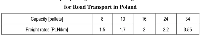
It is very difficult to build a model that would mirror the relationship between a delivery quantity and costs of transport. Table 2 presents exemplary freight rates for hiring road vehicles of different capacities for standard (not specialized) services. The method of calculating transportation expenditures in the case of external operators is very simple: the prices per kilometer (km) are multiplied by the number of km. The prices in Table 2 can be treated as typical, but they are not the same in all cases.
Table 2
Exemplary Freight Rates for Hiring Vehicles for Road Transport in Poland
Capacity [pallets] 8 10 16 24 34
Freight rates [PLN/km] 1.5 1.7 2 2.2 3.55
Source: Data collected in transportation market in Poland in year 2008
In Poland, the prices are market-based because the road transportation market is fully liberal as far as prices are concerned, but the level of rates depends on many factors, not only the capacity of the vehicles. For example:
•
On longer distances, rates per km are lower.•
On some transport connections, prices can be higher if it is hard to find return loads.•
In some cases, a driver accepts an extremely low price when he cannot find an order for the return trip and would otherwise have to wait or return with an empty truck.International Journal of Business and Information
•
The statutory working hours of a driver also influence rates. On good roads in the European Union (EU), a driver can travel 800 km during one work day, but after that, a 10-hour break is required.These are reasons the rates per km for a given type of vehicle are not the same in all cases. Quite often, carriers make their offer, not per km, but for the whole route. There are other reasons as well. Prices depend also on the type of service provided. When an operator offers a higher level of transportation service, the operator can negotiate a better freight rate. Another factor that influences rates is the level of specialization. A company that carries specialized loads (for example, refrigerated cargo) can obtain better prices than a company that transports loads that do not require special treatment. Even loads such as electronic devices can be priced better because they require vehicles with more space than normal ones.
Just after Poland’s accession to the European Union in 2004, rates fell by
20-30%. The reason was the elimination of customs clearance at borders and the opening of markets elsewhere in Europe. As a consequence, there was a larger supply of transportation services because more companies were able to carry more loads in a shorter time. Productivity is now higher, but rates are lower. What is interesting, however, is that not every company was forced to decrease prices. Some have sustained their rates, and others, such as couriers, have even raised them.
So, rates can change indiscreetly, along with a change in the size of a delivery, although the problems discussed above concern only one mode of transportation. In Poland, when the quantity of a delivery increases over 24-29 tons, a more massive mode of transport is used. In that case, costs change, also non-linearly. What is more, it is not profitable to use only a few rail wagons instead of a truck, because rail rates for small customers are not attractive. The main Polish rail carrier, PKP Cargo, however, offers big rebates (in some cases, up to 80%) for shippers who sign an agreement for regular transport of big shipments. This situation is even more difficult to consider in a mathematical function.
opinion, it does not make sense to use an average rate to solve the problems of a specific company.
The freight rates shown earlier in Table 2 are those that occur most frequently in the Polish market, but they cannot be used to create a universal model of the relationship between quantity decisions and transportation costs. Each company has specific conditions in which it operates. A separate model, therefore, could be established, for example, not only for a concrete company, but also for a concrete transport connection. It is very doubtful that such an aggregate model could serve as a useful decision-making tool in optimization formulas. More likely, the best method for finding optimal (or close to optimal) solutions is simulation, which, admittedly, is more labor- and time-intensive, but also more effective. Simulation seems to be more adequate for solving problems in complex logistics systems. The classical EOQ formula would probably be most useful in materials management, to solve problems of replenishing materials for production, where use is stable. For a few kinds of goods, transport is organized by the supplier.
The necessity of including transportation costs in the total logistic calculation becomes evident when a receiver of purchased goods has the transportation responsibility, or when transportation is organized within an internal logistic chain; e.g., from a factory to a company’s own warehouse. Such a situation occurs in the case of ZCh Police.
Transportation costs influence the logistics decision; namely, higher transportation costs encourage companies to supply goods in larger quantities. In this regard, one faces an interesting phenomenon: the optimal order quantity is a function of transportation and inventory costs, but transportation costs are also a function of order quantity. This situation is the reason, in some cases, that fixed transportation costs for one delivery cannot be placed into an EOQ formula (as it is with unit ordering costs), because the unit transportation costs (per 1 pallet or ton) are not fixed and depend on the number of goods that are transported. This problem will also be explained in the numerical example.
International Journal of Business and Information
Table 3
Unit Freight Rates for Deliveries from Plant to a ZCh Police Distribution Center [PLN/t]
Distribution Center 24 t >300 t >500 t >1,000 t >1,500 t
BALTIC STEVEDORING COMPANY - Szczecin 3.5 2.8 2.5 1.8 1.5
DAAR sp. z o.o. – Kunów 114 98 75 60 50
POLGAZ sp. z o.o. - Rypin 68 59 45 35 30
AMPOL- MEROL – Wąbrzeźno 68 59 45 35 30
SUPRA sp. z o.o. – Wrocław 84 72 55 40 30
SZEPIETOWO – Szepietowo 137 117 90 75 60
Source: The author’s calculations, based on data collected from transportation market in Poland.
Table 4
Freight Rates for Deliveries from Plant to a Zch Police Distribution Center [PLN]
Distribution Center 24 t >300 t >500 t >1,000 t >1,500 t
BALTIC STEVEDORING COMPANY - Szczecin 84 840 1,250 1,800 2,250
DAAR sp. z o.o. – Kunów 2,739 29,348 37,500 60,000 75,000
POLGAZ sp. z o.o. - Rypin 1,643 17,609 22,500 35,000 45,000
AMPOL- MEROL – Wąbrzeźno 1,643 17,609 22,500 35,000 45,000
SUPRA sp. z o.o. – Wrocław 2,009 21,522 27,500 40,000 45,000
SZEPIETOWO – Szepietowo 3,287 35,217 45,000 75,000 90,000
Source: The author’s calculations, based on data collected from the transportation market in Poland
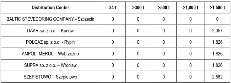
The question is: Which cost should be used as the cost of one delivery? The only solution seems to be to calculate several EOQs – each corresponding to a different delivery quantity.
several trucks would have to be sent to this distribution center. The EOQs for other distribution centers are even higher. For these centers, the possible EOQ’s
are those calculated with a quantity of > 1,500 tons, as shown in Table 6. As for the first distribution center, the best solution seems to be to deliver in quantities of at least 300 tons, because this quantity is close to the EOQ of 249 tons (EOQ calculated with the rate for delivery quantity >300 tons).
Table 5
Economical Order Quantities (EOQs) for Different Levels of Deliveries (Tons)
Distribution Center 24 t >300 t >500 t >1,000 t >1.500 t
BALTIC STEVEDORING COMPANY - Szczecin 79 249 304 365 408
DAAR sp. z o.o. – Kunów 450 1,474 1,667 2,108 2,357
POLGAZ sp. z o.o. - Rypin 349 1,142 1,291 1,610 1,826
AMPOL- MEROL – Wąbrzeźno 349 1,142 1,291 1,610 1,826
SUPRA sp. z o.o. – Wrocław 386 1,263 1,427 1,721 1,826
SZEPIETOWO – Szepietowo 493 1,615 1,826 2,357 2,582
Source: The author’s calculations, based on data collected from transportation market in Poland
Table 6
Corrected Economical Order Quantities (EOQs) for Different Levels of Deliveries (Tons)
Distribution Center 24 t >300 t >500 t >1,000 t >1,500 t
BALTIC STEVEDORING COMPANY - Szczecin 0 0 0 0 0
DAAR sp. z o.o. – Kunów 0 0 0 0 2,357
POLGAZ sp. z o.o. - Rypin 0 0 0 0 1,826
AMPOL- MEROL – Wąbrzeźno 0 0 0 0 1,826
SUPRA sp. z o.o. – Wrocław 0 0 0 0 1,826
SZEPIETOWO – Szepietowo 0 0 0 0 2,582
Source: The author’s calculations, based on data collected from transportation market in Poland
International Journal of Business and Information
5.
OPTIMAL DELIVERY SIZES IN DISTRIBUTION SYSTEM
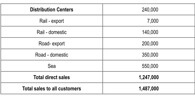
In this section, the problem discussed above is extended to a situation involving a distribution center that is part of a distribution system in which the factory warehouse for ZCh Police supplies 6 distribution centers and the rest of
the company’s direct customers in Poland and abroad. The distribution of sales
through different modes of transportation is shown in Table 7.
Table 7
Yearly Sales of ZCh Police Through Different Distribution Channels (Tons)
Distribution Centers 240,000
Rail - export 7,000
Rail - domestic 140,000
Road- export 200,000
Road - domestic 350,000
Sea 550,000
Total direct sales 1,247,000
Total sales to all customers 1,487,000
Source: Data from ZCh Police (year 2008)
In order to solve such a complex problem, the author constructed a more complex and more detailed model for use in the next stage of simulation. The model reveals three vertical and horizontal relationships between:
Products
Receivers of products (distribution centers, direct customers)
Links in the logistics-production chain (receivers, factory warehouse, production system, raw material warehouse)
arrival, or orders from the best customers would be served first. Neither situation, however, changes the fact that there is an interrelationship among receivers of products. A decision made by one receiver can affect other receivers. The thesis can be posited as follows:
Because decisions made at local distribution centers can influence other parts of the logistics–production system, the optimal parameters of deliveries for these centers will probably not be optimal from the point of view of the benefits of the whole system. This fact means that the EOQ model is inadequate for solving complex problems.
The computer program was applied, in which the following mathematical model was used:
o k n j z r k r I k j FV k j FI p l k l j LS k l j T m i k i j LS k i j T k i j IL C C C C C C C C
C
1 1 1 1 1
Where:
K – a specific day in which parameters of processes (e.g., level of inventories) are observed
j – number of products
i – number of distribution centers
l – number of customers
k i
j I
C
– costs of keeping inventory of j product in i distribution centre in k dayk i
j T
C
– transport costs to i distribution centerk i
j LS
C
– costs of lost sales of j product in i distribution centerk l
j T
C – transport costs to l customer
k l
j LS
C
– costs of lost sales of j product for l customerk j FI
C – costs of keeping inventory of j product in k day in factory warehouse
PF
C
– production fixed costsk j FV
International Journal of Business and Information k
r I
C
– costs of keeping inventory of r raw material in k day in raw materials factory warehouseRaw materials such as nitrogen (N), phosphate (P2O5), potassium (K2O), sulphur (S), and magnesium (MgO) comprise 58% of a final product and are estimated at the level of 200 PLN per 1 ton.
Costs of production are fixed and variable (manufacturing and raw materials). A total of 12 products are produced in the Zch Police manufacturing system, the capacity of which is a maximum of 10,000 tons daily, with an average daily production of 6,000 tons. The yearly fixed costs of such a system are 220 mln PLN. The model has the possibility of increasing this capacity, but, in that case, production costs would also be increased.
Because the change-over time every day is long (0.5 – 3 hr.), only two products can be produced. This means that a big portion of the daily production is made for stock.
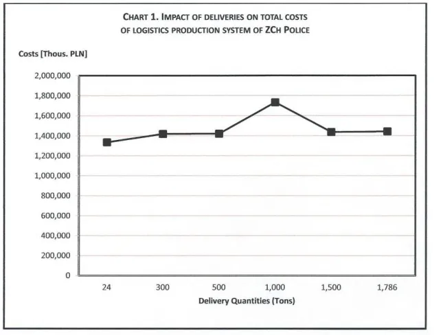
The results of these simulations are shown in Table 8 and in Chart 1. The quantities sent to distribution centers are like those in previous calculations: 24 (road transport), 300, 500, 1,000, and 1,500 tons. The last column of Table 8 presents the optimal quantities calculated for each distribution center, from Table 6. The costs corresponding to the quantities are 1,442 mln PLN, which is not the lowest. These sizes of deliveries are not optimal for either the whole system or the distribution centers. The optimal size for deliveries to the distribution centers is 500 tons. For the whole system, however, the total costs are 1,421 mln PLN. In fact, the lowest level of costs for the whole system (“optimal system strategy”) is obtained when the products are sent by 24-ton trucks, in which case, the costs are 1,335 mln PLN.
It should yet be stressed that the result when the last option is applied is not
the worst one. The worst is “1,000 tons OQ” strategy (costs: 1.7 mln PLN).
The saving that results from the difference between “optimal distribution
centers”and “optimal system,” however, is considerable: 0.86 mln PLN. Perhaps
Table 8
Logistics and Production Costs for Different Variants of Deliveries for ZCh Police (Thous. PLN)
Delivery Quantity (tons) 24 300 500 1,000 1,500 1,786
Production costs 1,277,825 1,404,047 1,406,466 1,715,701 1,409,570 1,409,028
Costs of inventories and warehousing
of raw materials 2,536 902 916 917 1,547 1,345
Costs of inventories and warehousing
in the factory warehouse 43,111 10,610 10,921 11,674 21,535 19,633 Costs of direct deliveries to customers 90,946 90,615 91,245 91,445 91,258 91,512
Costs of lost sales 19,051 19,051 19,051 19,051 19,051 19,051
Inventory and warehousing costs in
distribution centers 234 737 1,247 2,506 3,730 11,147
Transportation costs to centers 11,714 2,880 2,261 1,751 703 1,347
Costs of supplying the centers 11,948 3,617 3,508 4,257 4,433 12,494
Total costs 1,335,420 1,419,176 1,421,810 1,732,549 1,437,085 1,442,500
International Journal of Business and Information The reasons for these differences can be explained by analyzing what happens on the level of the distribution centers and the level of the factory. Table 9 shows the impact of changes in the delivered quantities to distribution centers on the logistics and production potential of the whole chain.
Table 9
The Influence of Delivery Sizes to Distribution Centers on Logistics and Production Processes at ZCh Police (Tons)
Delivery Quantity (Tons) 24 300 500 1,000 1,500 1,786
Reorder point 50 50 50 50 50 50
Average raw material level 18,851 19,148 19,155 32,294 28,097 28,305
Average level of inventory in
factory warehouse 220,165 226,606 242,234 446,861 407,389 477,101 Average level of inventory in
distribution centers 3,417 10,803 18,308 37,027 55,078 69,669 Required production capacity 8,420 10,667 11,970 22,890 17,348 18,241
Required reloading capacity in factory 15,941 19,234 14,909 22,283 20,455 30,120
Required reloading capacity in
distribution centers 1,728 9,108 14,500 22,000 24,000 35,031
As shown in Chart 2 and Chart 3, the factory has to build the proper potential to fill the orders of its distribution centers.
Smaller and more frequent orders sent from distribution centers and other receivers make factory functionality more stable. This means that the factory has to build a lower logistics potential because the orders are smaller. For ZCh Police, inventories increased when delivery sizes were larger, not only at the distribution centers, but also at the factory. The reason, of course, is the higher amplitude of fluctuations in the quantity of orders from the distribution centers.
The consequence of changing the production level is a change in the supply area – levels of raw materials inventories also increase.
International Journal of Business and Information Source: Author of this paper
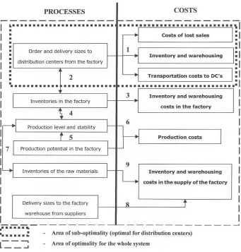
Figure 2. Model of Relationship Processes and Their Economical Efficiency
Following is an explanation of the relationships shown in the figure.
2. Orders sent to the factory warehouse influence the level of product inventories in the factory warehouse. The level of these inventories, however, influences the actual sizes of deliveries to the distribution center, which can, in fact, be lower than the orders. That is why it is a two-way relationship. As a consequence, the actual customer service level of the distribution center can differ from the expected one.
3. The level of inventories in the factory warehouse influences the costs of keeping them.
4. The relationship between these inventories and the level of production and its stability is also two-directional: the decrease in inventory level triggers an increase in production. Frequent changes in the level of inventories can cause production to become unstable. On the other hand, if production does not change much, shortages of inventories can occur, which will result in a lower level of service.
5. The level of production depends on production potential. If production is low, the production system cannot flexibly adjust to changes in inventories.
6. Production processes and production potential impact production costs. 7. Production level depends not only on production resources, but also on
the availability of inventories of raw materials. Unstable production also causes changes in the level of these inventories.
8. Raw materials inventories also depend on the size of deliveries from suppliers.
9. Raw materials inventories affect their costs.
The preceding analysis reveals that economical efficiency is the result of a combination of main factors: orders from the distribution centers, production potential, and the size of the deliveries of raw materials from suppliers.
6.
CONCLUSIONS
International Journal of Business and Information of processes at the factory level. This finding indicates that it would be worthwhile to conduct further research on the optimization of complex systems.
Simulations conducted during this study showed that it is not easy to find a model that can serve effectively as a decision-making tool to solve the problem of economical order quantity (EOQ), especially in complex logistics systems. In some cases, the classical EOQ formula could be inappropriate for at least two reasons.
First, the EOQ formula reflects a trade-off between ordering costs and inventory-warehousing costs at one point in the logistics chain. In other words, the formula reflects the impact on a limited number of processes and costs, although other processes are involved that are not included in the formula. The model presented in this paper shows trade-offs that exist in the relationships among the several parts of a logistics system – distribution centers, central warehouse, factory, and supply of materials. Also, customers have their own preferences concerning delivery strategies. The optimal solution is one that provides the maximum advantages from the point of view of the whole system, not just one element of the system (sub-optimality).
The second reason the classical EOQ could be inappropriate involves the phenomena of non-linear relationships between logistics processes and their effectiveness, which should be captured in a model if that model is to serve as a useful decision-making tool.
When the complexity of logistics problems is taken into account, it is very likely that, in practice, models that are developed for simulations can be more useful than optimization formulas.
More variants of the model could be used; for example, to include the impact of production strategies. In the case study in this paper, production was assumed to be stable (“make to stock” strategy), which means that, in order to meet changing demand, some level of stock has to be built. The impact of changing replenishment sizes to distribution centers would probably be stronger in the case of the “make to order” production system than in the case of the
for implementing the “made to order” concept is reduction of change-over times in production.
Different distribution strategies could also be tested. In this paper, only one reactive system was considered (PULL distribution). Every time the level of inventories in the distribution centers or for direct customers was lower than reorder point, the orders were sent to the factory for replenishment. In a company like ZCh Police, a better solution would perhaps be a PUSH system based on delivery schedules. That system could be coupled with consolidation of the deliveries of products in order to reduce transportation costs. When an ideal PULL system is implemented, orders for individual products could be sent at different times, which would make it difficult to consolidate shipments. A PUSH strategy could probably stabilize the functioning of the factory. There is also a chance that lead time (in this variant, it was 3 days) could be shorter. When deliveries are scheduled, many operations can be planned earlier, which would help increase the efficiency of these operations. A transportation operator, for example, could be informed earlier about transportation requirements, which could help the operator provide better service and could also lead to a reduction in transportation costs.
The question, however, is whether such consolidation is possible. The products of ZCh Police are chemical goods – some would say, hazardous goods –
a fact which raises the question of whether such products should be transported together. Certainly, a thorough investigation should be made before attempting such consolidation. Since every receiver does not need an assortment of fertilizers, however, it may be possible to consolidate certain products.
In summary, if mathematical optimization models are to solve practical problems, these models should consider concrete, practical circumstances relating to the problems. The models should also include many factors – first of all, the relationships between logistics and other areas. It may be that, rather than looking for one general, universal model, one should instead construct different models that mirror different optimization problems.
REFERENCES
Baumol, W.J., and Vinod, H.D. 1970. An inventory theoretic model of freight transport demand, Management Science 16, 413-421.
International Journal of Business and Information Constable G.K., and Whybark D.C. 1978. The interaction of transportation and
inventory decisions, Decisions Science 9, 688-699
Cordeau, Jean-Francois; Pasin, Federico; Salomon, Marius M. 2003. An integrated model for logistics network design, Annals of Operations Research.
Das C. 1974. Choice of transport services: An inventory–theoretical approach, Logistics and Transportation X, 181-187.
Ferguson W., and Glorfeld L.W. 1981. Modeling the present motor carrier rate structure as a benchmark for pricing in the new competitive environment, Transportation Journal 21, 59-66.
Fokkens B., and Puylaert M. 1981. A linear programming model for daily harvesting operations at the large-scale grain farm of the IJsselmeerpolders Development Authority, Journal of the Operational Research Society 32(7), 535-547.
Langley, C.J. 1980. The inclusion of transportation costs in inventory models: Some considerations, Journal of Business Logistics 2, 6-125.
Madadi, Alireza; Kurz, Mary E.; Ashayeri Jalal. 2010. Multi-level inventory management decisions with transportation cost consideration, Transportation Research Part E 46, 719-734.
Milewski, D. 2006. The logistics models as tool for optimization of complex logistics problems, Gospodarka Materiałowa &Logistyka, No. 7-8.
Milewski D. 2007. The relation between the size of a delivery and safety stocks. Gospodarka Materiałowa &Logistyka, No. 1.
Milewski D. 2007. Optymalizacja dostaw w sieci dystrybucji, Gospodarka Materiałowa & Logistyka, No. 1.
Milewski D. 2009. The optimization of deliveries in distribution of foods – The choice between PULL and PUSH strategy, Gospodarka Materiałowa &Logistyka , No. 12. Meyer J.R.; Peck, M.J.; Stenason J.; and Zwick, C. 1959. The Economics of Competition in the Transportation Industries, Cambridge, MA: Harvard University Press.
Mutlu, Fatih, and Çetinkaya, Sıla. 2010. An integrated model for stock replenishment and shipment scheduling under common carrier dispatch costs, Transportation Research Part E 46.
Prasad H.V.V., and Sankaran, Jayaram K. 1996. Optimization-based distribution planning for consumer electronic items, Journal of Operational Research Society 47(7), 895-905.
Ryu, W., and Lee, K.K. 2003. A stochastic inventory model of dual-sourced supply chain with lead-time reduction, International Journal of Production Economics, 81-82, 513-527.
Symposium on Intelligent and Evolutionary Systems, Clayton, Victoria, Monash University, 162-170.
Stenger, Alan J.; Coyle, John J.; and Price, Marshall S. 1977. Incorporating transportation costs and services into inventory replenishment decisions, In: Applied Distribution Research, Robert G. House and James F. Robeson (eds.), Columbus, Ohio: Ohio State University, pp. 22-26.
Swenseth, S.R., and Godfrey, M.R. 1996. Estimating freight rates for logistics decisions, Journal of Business Logistics 17(1).
Zhao, Qiu-Hong; Wang, Shou-Yang; Lai, K.-K.; and Xia, Guo-Ping. 2004. Model and algorithm of an inventory problem with the consideration of transportation cost, Computers & Industrial Engineering 46, 389-397.
ABOUT THE AUTHOR
Dariusz Milewski has been a scientific worker and lecturer at the University of Szczecin