©2017 JNAS Journal-2017-6-2/39-51 ISSN 2322-5149 ©2017 JNAS
A Multistep Broyden’s-Type Method for Solving
System of Nonlinear Equations
M.Y.Waziri
1*, M.A. Aliyu
2and A.Wakili
31- Department of Mathematical Sciences, Faculty of Sciences, Bayero University, Kano, Kano State, Nigeria
2- Department of Mathematical, Faculty of Scienves, Gombe State, Gombe State
3- Department of Mathematical Sciences, Faculty of Sciences, Federal University, Lokoja, Koji State, Nigeria
Corresponding author:
M.Y.Waziri
ABSTRACT: The paper proposes an approach to improve the performance of Broyden’s method for solving systems of nonlinear equations. In this work, we consider the information from two preceding iterates rather than a single preceding iterate to update the Broyden’s matrix that will provide sufficient information in approximating of the Jacobian matrix in each iteration. Under some suitable assumption, the convergence analysis is established. The numerical results verify that the proposed method has clearly enhanced the numerical performance of Broyden’s Method.
Keywords: Multi-Step Broyden, nonlinear systems of equations, Performance profile. INTRODUCTION
Solving systems of nonlinear equations is becoming more essential in the analysis of complex problems in many research areas. The problem considered is to find the solution of nonlinear equations
(x)
0,
F
(1)Where
:
n n
F D
has continuous first partial derivatives. The assumption here is there exist a vector
* * * *
1
,
2,
,
nx
x x
x
with
*
0
F x
and
*
0,
F
x
where
F
x
k is the Jacobian matrix ofF
atx
k isassumed to be locally Lipschitz continuous at
x
*.
Newton’s method is a well know method for solving
(1).
The method generates an iterative sequence
x
k from a given initial guessx
0 via1
1
(
)
(
)
k k k k
x
x
F x
F x
(2)
where
k
0,1,2
.
However, despite the fact that the Newton’s method is simple to implement and has a quadratic rate of convergence, still it requires the computation and storage of
n n
Jacobian matrix and its inverse, and also requires solving systems of linear equations at each iteration. In practice, computations of some functions derivatives are quiet costly and sometimes they are not available or could not be done precisely. In this case, Newton’s method cannot be used directly.40
Jacobian matrix and its inverse by a derivative free matrix (known as Broyden’s matrix) and therefore calculating the derivative in every iteration is avoided.
Broyden’s method uses the information from the last iterate to compute the current point which makes it has lesser information of the previous iterates. It will be nice if we can incorporate the information of the last two or more iterates and update the Broyden’s matrix. By doing this, the Broyden matrix will have sufficient information from the previous iterates and hence improve the accuracy of the Jacobian approximation. This motivated the paper.
Waziri et al [10] incorporated the concept of two-step into diagonal updating and solve system of nonlinear equations and they succeeded in enhancing the method developed by Leong et al [15]. The main reason for developing this approach is to improve the accuracy Broyden’s matrix via multi-step in which we use the information from two preceding iterates to compute the current point. This paper is organized as follows: the next section describes our new approach; section 3 gives the convergence analysis of our proposed method. The numerical results are presented in section 4 and the conclusion is given in section 5.
1. MULTI-STEP BROYDEN-LIKE APPROACH
This section describes our new multi-step Broyden-like approach which generates a sequence of vectors
x
k via
1
1
,
k k k k
x
x
B F x
(3)
Where
B
k is the Broyden approximation of the Jacobian matrix updated in each iteration via multi-step approach.Our target is to come up with a matrix
B
k through a Broyden updating scheme. To achieve this, we make use of aninterpolating curve in the variable space to develop a modified secant equation which was derived initially by Dennis and Wolkowicz [3]. This is made possible by considering some of the most successful two-step methods [5,4,9,6] for more detail. Through integrating this two-step information, we can present an improve secant equation as follows:
1 1 1
k k k k k k k
B
s
s
y
y
(3)
By letting
k
s
k
k ks
1 and
k
y
k
ky
k1 in (4), we have ,k k k
B
(4)
Since we incorporate the information from the last two preceding iterations instead of a preceding iteration in (4) and
(5), we require to build an interpolating quadratic curves
x v
andy v
,
wherex v
interpolates the last twopreceding iterates
x
k1 andx
k,
andy v
interpolates the last two preceding function evaluationF
k1 andF
k.
Using the approach introduced in [5], the value of
k in (4) can be determine by computing the values ofv v
0,
1 and 2.
v
By lettingv
2
0,
20
j j
v
can be computed as follows:
1 2 1
2 1
1
1 2
=
( )
( )
=
=
=
k
k k
k k k
T k k k
v
v
v
x v
x v
x
x
s
s B s
B
B
B
41
0 2 0
2 0
1 1
1
1 2
1 1
=
( )
( )
=
=
=
k k k
k k k k
T
k k k k k
v
v
v
x v
x v
x
x
s
s
s
s
B s
s
B
B
B
(6)
Let us define
k by2 0
1 0
,
k
v
v
v
v
(7)
Therefore
k and
k can be computed by the following relations2
1
,
1 2
k
k k k
k
s
s
(8)
2
1
,
1 2
k
k k k
k
y
y
(9)
That is,
k in (4) is given by
2
1 2
.
k k k
Using the same approach as in [10] and considering the Broyden’s update as in [8], the Multi-Step Broyden’s matrix is obtained as
1
T k k k k
k k T
k k
B
B
B
(10) Now, the algorithm for our method is as follows;
Algorithm 2.1 (Multi-Step Broyden’s method (MSBM))
0
1:
n: 0
Step
Choose an initial guesss
e
t
B
I and let
k
42 :
(
k).
(
k)
,
10 .
Step
Compute F x
If
F x
stop where
1
1 0 0 0
3:
: 0
( ).
: 1
k k k k5.
Step
If k
define x
x
B F x
Else if k
set
s and
y and go to
1 0 4
2 2
4 :
2
,
(6) (8)
(9)
(10)
.
10
.
k k k
T
k k k k k k k k
Step
If k
compute v v and
via
respectively and find
and
using
and
respectively If
set
s and
y
1
1 1
5:
k k k(
k)
k(11).
Step
Let x
x
B F x
and update B
as defined by
1 1 .
2
v6 :
k
,
k,
5.
,
k kStep
Check if
if yes retain B
that is computed by step
Else set B
B
7:
:
1
2.
Step
Set k
k
and go to
2. CONVERGENCE ANALYSIS
This section discusses the convergence analysis of our method. The following theorem is stated without proof as it will be useful in proving the superlinear convergence of the Multi-step Broyden update.
Theorem 3.1 [14]. Let
F
:
n
n be continuously differentiable in an open, convex set D in,
n
and assume
that for some
x
* in D,F
is continuous atx
* andF x
( )
is nonsingular. LetB
kin
n
L
42
nonsingular matrices and suppose for some
x
0 in D the iterates generated by1
1
(
),
k k k k
x
x
B F x
x
k remains inD and converges to
x
* at a superlinear rate if and only if
'
1
1
(
)
lim
k k k0.
k
k k
B
F x
x
x
x
x
Now, we show the superlinear convergence of our methodTheorem3.2 Let
F
:
n
nbe continuously differentiable function in an open convex setC
.
Assume that there exist positive constants
and
such thatx
0x
and
'
0
(
)
.
B
F x
Then the sequence
x
k generated by Multi-step Broyden’s update1
1
(
)
k k k k
x
x
B F x
(11)
1
T k k k k
k k T
k k
B
B
B
(12)
is well define and convergence to
x
* superlinearly.Proof: By theorem (3.1), it is enough to show under the conditions of the theorem that
'
1
1
(
)
lim
k k k0
k
k k
B
F x
x
x
x
x
(13) From (12) and (13),
1
(
)
(
)
(
)
(
)
=
(
)
(
)
=
(
)
T k k k k
k k T
k k
T T
k k k k k k k
k T T
k k k k
T T
k k k
k k
k T T
k k k k
B
B
F x
B
F x
F x
B
F x
B
F x
F x
B
F x
I
(14)Taking norms on both sides gives
1
(
)
(
)
(
)
T k k k kk k T
k k k
F x
B
F x
B
F x
I
(15) Since1
T k k T k kI
(16)
And by the fact that
( )
( )
( )(
)
2
F u
F v
F x u v
u
x
v
x
u v
We have
1 1(
)
(
)
(
)
(
)
2
k
F x
kF x
kF x
kF x
kx
kx
x
kx
k
(17)Hence
1
(
)
(
)
1.
2
k k k k
B
F x
B
F x
x
x
x
x
43
Now let
E
kB
kF x
(
).
From (16), we have
1(
)
T T
k k k
k k F
k F k T T
k k F k k
F x
E
E
I
(18) Since
2 42 2 2
2
4 4 2
=
=
=
TT T T
k k k k k k k k
k T T T
k k F k k k k
T T
k k k k k k k
k k T k k k k
k k k
k k k
E
E
E
tr
E
E
tr
E
E
E
tr
And=
T T T T
k k k k k k k k
k k T k k T k T k T
k k k k k k k k
E
E
E
E
E
E
I
We get
,
T Tk k k k
k k T k T
k k k k
tr E
tr E
E
I
that is,2 2
2 k kT k Tk
k F k T k T
k k F k k F
E
E
E
I
Therefore 2 2 2 2 Tk k k k
k F k T
k k
k F
E
E
E
I
Hence 1 2 2 2 2 T k k k kk T k F
k k F k
E
E
I
E
(19)Since
2 2 2
2
for any
0,
(20) implies that2 2
.
2
T k k k kk T k F
k k F k F k
E
E
I
E
E
(20)Now, by using (21), (18), and the fact that
1
1
0.
2
k k
x
x
x
x
k
(21)
We can write (19) as
2 1 2
3
,
4
2
k kk F k F k
k F k
E
E
E
x
x
E
which is 2 1 23
2
4
k kk F k F k F k k
E
E
E
E
x
x
44
But from
(
)
2 2
k k
B
F x
and (22), we have that
E
k F
2 ,
k
0
and 02 .
k k
x
x
Thus, (23) can be written as
2
1 2
3
4
.
4
k kk F k F k
k
E
E
E
x
x
(23) By summing both sides, we obtain
2
0 1
2
0 0
0
0
3
4
4
3
4
2
3
4
,
2
i i
k k
i k
F F
k k k
F F
E
E
E
x
x
E
E
Which hold
i
0.
Therefore2
2 0
0
k k k k
k k k
E
E
as
k
.
Hence the proof is complete. 3. NUMERICAL RESULTSIn this section, we analyze and compare the performance of MSBM with that of Newton’s method NM, Fixed Newton’s method FNM and Broyden’s method BM for solving systems of nonlinear equations. The algorithms are written in MATLAB7.10.0 (R2010a) and are tested for some classical benchmark problems. All the problems were run on a PC with AMD E1-1200APU with Radeon(tm) CPU with 2.00Ghz speed. To describe the results of these experiments we give the dimension of problem (N), the number of iterations performed(NI) and the CPU time (seconds).
We declare a termination of the methods whenever,
4
(
k)
10
F x
(24)
The identity matrix has been chosen as an initial approximate Jacobian. The symbol
" "
is used to indicate a failure due to:(1) The number of iteration is at least 500 but no point of
x
k that satisfies (12) is obtained;(2) CPU time in second reaches 500; (3) Insufficient memory to initiate the run.
Dolan and More´[2] gave a new tool of analyzing the efficiency of Algorithms. They introduced the notion of a performance profile as a means to evaluate and compare the performance of set of solvers S on a set P. Assuming
there exist ns solvers and np problems, for each problem p and solvers s, they defined
t
p s,
computing time (the number of function evaluations or others) required to solve problem p by solvers s.Requiring a base line for comparisons, they compared the performance on problem p but solver s with the best performance by any solver on this problem; using the performance ratio
, ,
,
min
:
p s p s
p s
t
r
t
s
S
(25)
Suppose that a parameter
r
M
r
p s, for allp s
,
is chosen, andr
p s,
r
M if and only if s does not solve problem p.The performance of solver s on any given problem might be of interest, but we would like to obtain an overall assessment of the performance of the solver, then they defined
,
1
( )
:
s p s
p
t
sizep
P r
t
n
45
Thus
s( )
t
is the probability for solvers
S
that a performance ratior
p s, is within a factort
R
of the bestpossible ration. Then function
s is the (cumulative) distribution function for the performance ration. Theperformance profile
s:
R
0,1
for a solver is a nondecreasing, piecewise constant function, continuous from the right at each breakpoint. The value of
s(1)
is the probability that the solver win over the rest of the solvers.According to the above rules, we know that one solver whose performance profile plot is on the top right will win over the rest of the solvers.
Below are the benchmarks problems used to test the proposed methods in this research. problem 1(Artificial Function)
2
0
( )
cos
1
1,
1,2,
, and
0.5, 0.5,
, 0.5
Ti i
f x
x
i
n
x
problem 2(Trigonometric system of Beyong, 2010)
0
( )
cos
1,
1, 2,
, and
0.5, 0.5,
, 0.5
Ti i
f x
x
i
n
x
problem 3(Beyong et al, 2010)
1
1 0
( )
1,
( )
+1,
1, 2,
, and
0.5, 0.5,
, 0.5
i i i
T
n n
f x
x x
f x
x x
i
n
x
problem 4(Artificial Function)
0
( )
sin
cos
cos
1
,
1, 2,
, and
0.5, 0.5,
, 0.5
Ti i i i i i i
f x
x
x x
x
x
x
i
n
x
problem 5(Beyongetal, 2010)
2
0
( )
1,
1, 2,
, and
0.5, 0.5,
, 0.5
Ti i
f x
x
i
n
x
problem 6
1 2 2 1
1 0
( )
sin
4exp 2
2 ,
( )
sin 2
4exp
2
2 +cos 2
exp 2
,
1, 2,
, and
0.5,0.5,
,0.5
iT
n i i i i
f x
x
x
x
x
f x
x
x
x
x
x
i
n
x
problem 7(Artificial Function)
2
1 0
( )
1
1
2
2,
1,2,
, and
0.5,0.5,
,0.5
Ti i i i n n n
f x
x
x
x x
x x
i
n
x
problem 8(Darvishi and Shin, 2011)
0
( )
xi1,
1, 2,
, and
0.5, 0.5,
, 0.5
Ti
f x
e
i
n
x
problem 9(Artificial Function)
1 1
1 0
( )
,
( )
cos
+
1,
1, 2,
, and
2, 2,
, 2
Ti i i
f x
x
f x
x
x
i
n
x
problem 10(Beyong, 2011)
2
0
( )
4,
1, 2,
, and
2.5, 2.5,
, 2.5
Ti i
f x
x
i
n
x
problem 11(Beyong, 2011)
2
0
( )
2,
1, 2,
, and
0.5, 0.5,
, 0.5
Ti i i
f x
x
x
i
n
x
problem 12(Artificial Function)
2 1
1 1
2 1
1 0
( )
4
2
,
3
( )
4
2
,
1, 2,
,
1 and
0.5, 0.5,
, 0.5
3
i
i i i
T n
n n n n
x
f x
x
x
x
x
f x
x
x
x
i
n
x
46
problem 13(Artificial Function)
2
0
( )
3 log
3
9,
1, 2,
, and
0.9, 0.9,
, 0.9
Ti i i i
f x
x
x
x
i
n
x
problem 14(Artificial Function)
2
1
1 1 1
0
( )
cos
9 3
8
,
( )
cos
9 3
8
i,
1, 2,
, and
0.5,0.5,
,0.5
xT x
i i i
f x
x
x
e
f x
x
x
e
i
n
x
problem 15(Artificial Function)
2 2
1 0
( )
0.5
0.25
1,
1, 2,
, and
0.5, 0.5,
, 0.5
Ti i n i i
f x
x
x
x
i
n
x
problem 16(Hafizand Baghat, 2012)
2
0
( )
cos
1 ,
1, 2,
, and
0.5, 0.5,
, 0.5
Ti i i
f x
x
x
i
n
x
problem 17(Artificial Function)
0
sin
( )
3
0.66
2,
1, 2,
, and
0.5, 0.5,
, 0.5
3
T i
i i i
x
f x
x
x
i
n
x
problem 18(Artificial Function)
2
0
( )
exp
1
cos 1
,
1,2,
, and
0.5,0.5,
,0.5
Ti i i
f x
x
x
i
n
x
problem 19(Artificial Function)
2
2
0
( )
1
2,
1,2,
, and
0.5,0.5,
,0.5
Ti i
f x
x
i
n
x
Problem20(Rooseetal.,1990)
2 0 2 1 11
( )
+
,
1, 2,
, and
0.5, 0.5,
, 0.5
n n
T
i i i i
i i
f x
x
x
x
n
i
n
x
n
Problem21(System of n nonlinear equations)
0
1 1
( )
3
cos
2
+
sin
2
,
1, 2,
, and
2, 2,
, 2
n n
T
i i i i
i i
f x
n
x
x
x
i
n
x
Problem22(Trigonometric System)
21 1 1 1 2
2
1 0
( )
3
1 cos
,
( )
3
1 cos
,
1, 2,
, and
0.5,0.5,
,0.5
Ti i i i i
f x
x
x
x
x
f x
x
x
x
x
i
n
x
problem 23(System of n nonlinear equations)
2 2
1
2 2
1 0
( )
0.1
,
( )
0.1 ,
1, 2,
, and
0.5,0.5,
,0.5
i i i
T
n i
f x
x
x
f x
x
x
i
n
x
Problem24(System of n nonlinear equations)
2
0 1
1
1
( )
cos
sin
1
1
,
1, 2,
, and
0.5, 0.5,
, 0.5
n
T
i i i n i i i
i
f x
x
x
x
x
x
x
i
n
x
n
n
Problem25(System of n nonlinear equations)
2
1 1 2 1
2 1
2 1
0
( ) 2 log cosh 1 1,
( ) 2 log cosh 1 1,
( ) 2 log cosh 1 1,
1
1, 2, , 0.5, 0.5, , 0.5 10 and
1
i i i i
n n n n
T
f x x x uh x
f x x x uh x
f x x x uh x
i n x u h
47
Below we give the tables and graphs that show the performance of Multi-step Broyden method in comparison with Newton method (NM), Broyden’s method (BM) and Fixed Newton method (FNM). We denote by MSBM the method define in algorithm (2.1).
Table1. Numerical Results of the methods when solving problems 1-6
NM FNM BM MSBM
Problems N NI CPU Time NI CPU Time NI CPU Time NI CPU Time
P1 25 14 0.0547 - - 6 0.0001 4 0.0001
50 14 0.1388 - - 6 0.0312 4 0.0312
100 15 0.362 - - 6 0.1872 4 0.0468
500 16 17.9348 - - 7 1.2168 6 1.4196
1000 16 133.2068 - - 7 6.2088 6 7.1604
P2 25 15 0.0564 - - 10 0.0312 8 0.0312
50 16 0.1226 - - 10 0.0468 8 0.0312
100 16 0.3777 - - 11 0.156 8 0.1572
500 - - - - 11 1.8408 8 1.638
1000 - - - - 12 10.2337 8 8.5489
P3 25 5 0.0194 - - 5 0.0312 3 0.0001
50 - - - - 5 0.0648 3 0.0312
100 - - - - 5 0.0936 4 0.0314
500 - - - - 5 0.7644 4 0.9828
1000 - - - - 5 3.6348 4 4.524
P4 25 - - 15 0.0639 3 0.0312 2 0.0001
50 - - 16 0.1475 3 0.0312 2 0.0013
100 - - 16 0.5388 3 0.0312 2 0.0312
500 - - 17 18.5478 4 0.5928 3 0.7176
1000 - - 18 137.7307 5 3.4788 3 3.5568
P5 25 5 0.017 - - 5 0.0156 3 0.0312
50 5 0.0558 - - 5 0.0312 3 0.0312
100 5 0.1403 - - 5 0.0936 4 0.0468
500 5 5.601 - - 5 0.8112 4 0.8736
1000 5 40.1397 - - 5 3.5412 4 4.6956
P6 25 5 0.023 - - 7 0.0468 6 0.0312
50 5 0.0684 - - 7 0.156 6 0.0312
100 5 0.1726 - - 6 0.1092 5 0.156
500 5 5.5923 - - 7 1.17 5 1.1544
1000 5 38.6409 - - 6 4.7112 5 5.772
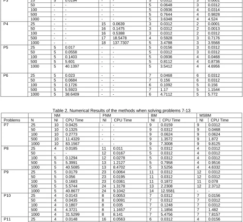
Table 2. Numerical Results of the methods when solving problems 7-13
NM FNM BM MSBM
Problems N NI CPU Time NI CPU Time NI CPU Time NI CPU Time
P7 25 10 0.0425 - - 9 0.0159 9 0.0312
50 10 0.1325 - - 9 0.0312 9 0.0468
100 10 0.2773 - - 9 0.0624 9 0.0624
500 10 11.4329 - - 9 1.3572 9 1.872
1000 10 83.1567 - - 9 7.3008 9 9.8125
P8 25 4 0.0185 11 0.011 5 0.0312 4 0.0312
50 - - 12 0.0167 5 0.0312 4 0.0312
100 5 0.1294 12 0.0278 5 0.0312 4 0.0312
500 5 5.3991 13 1.2127 5 0.7958 4 0.9516
1000 5 40.5085 13 8.4702 5 3.5256 4 4.6332
P9 25 5 0.0179 23 0.0064 11 0.0312 12 0.0312
50 5 0.056 23 0.0195 11 0.0312 12 0.0312
100 5 0.1683 23 0.0361 11 0.1872 11 0.078
500 5 5.5744 24 1.3178 13 2.2308 12 2.3712
1000 5 40.8677 24 9.1042 14 12.5581 - -
P10 25 4 0.0143 8 0.0053 7 0.0312 7 0.0156
50 4 0.0435 8 0.0091 7 0.0312 7 0.0312
100 4 0.1807 8 0.035 7 0.1248 7 0.0312
500 4 4.3721 8 1.1657 7 1.1856 7 1.482
1000 4 31.5299 8 8.141 7 5.4756 7 7.8157
P11 25 4 0.0148 16 0.0563 6 0.0312 4 0.0156
48
100 4 0.1523 17 0.0946 6 0.1092 4 0.0468
500 5 5.4596 18 1.1769 6 0.9984 4 0.9516
1000 5 36.5684 19 7.981 6 4.5708 4 4.6488
P12 25 4 0.0178 6 0.0067 5 0.0624 3 0.0001
50 4 0.0397 6 0.0106 5 0.1404 3 0.0156
100 4 0.1547 7 0.0266 5 0.1404 3 0.0312
500 4 4.2022 7 1.0869 5 0.7488 3 0.6864
1000 4 30.5035 7 7.6241 5 3.4164 3 3.6036
P13 25 4 0.0298 8 0.0098 6 0.0021 5 0.0012
50 4 0.0379 8 0.0326 6 0.0936 5 0.0312
100 4 0.1263 8 0.0379 6 0.1248 5 0.0468
500 4 4.7032 8 1.2449 6 0.936 5 1.0764
1000 4 32.4366 8 8.7337 6 4.7892 5 5.7408
Table 3. Numerical Results of the methods when solving problems 14-20
NM FNM BM MSBM
Problems N NI CPU Time NI CPU Time NI CPU Time NI CPU Time
P14 25 - - - - 8 0.0312 7 0.0312
50 - - - - 9 0.0624 7 0.0624
100 - - - - 9 0.078 7 0.0624
500 - - - - 9 1.5756 7 1.56
1000 - - - 7 7.8625
P15 25 6 0.0357 - - 6 0.0312 - -
50 6 0.0739 - - 6 0.0312 - -
100 6 0.1593 - - 6 0.0468 - -
500 6 6.7031 - - 6 0.9672 - -
1000 6 48.1997 - - 6 4.5552 - -
P16 25 6 0.0221 - - 5 0.0468 3 0.0156
50 6 0.0464 - - 5 0.0468 3 0.0312
100 6 0.1459 - - 5 0.0468 4 0.0312
500 6 0.0793 - - 5 0.6864 4 0.936
1000 6 48.0269 - - 5 3.6348 4 4.6956
P17 25 5 0.0439 - - 5 0.0156 4 0.0156
50 5 0.0572 - - 5 0.0312 4 0.0312
100 5 0.1859 - - 5 0.0312 4 0.0936
500 5 5.5123 - - 5 0.7332 4 0.9984
1000 5 41.1653 - - 5 3.5412 4 4.9296
P18 25 - - - - 6 0.0468 5 0.0021
50 - - - - 6 0.156 6 0.0312
100 - - - - 6 0.1872 6 0.0624
500 - - - - 7 1.0764 6 1.2948
1000 - - - - 7 5.46 6 6.8172
P19 25 - - - 6 0.0021
50 - - - 6 0.0156
100 - - - 6 0.0624
500 - - - 6 1.2636
1000 - - - 6 6.63
P20 25 4 0.0231 5 0.0728 6 0.0156 6 0.0156
50 3 0.0263 5 0.0145 6 0.0312 5 0.0312
100 3 0.1607 4 0.0292 6 0.0624 5 0.0312
500 3 3.3761 4 1.18837 6 1.0452 4 0.936
49
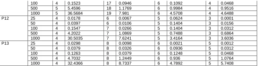
Table 4. Numerical Results of the methods when solving problems 21-25NM FNM BM MSBM
Problems N NI CPU Time NI CPU Time NI CPU Time NI CPU Time
P21 25 8 4.8507 - - 6 0.0468 4 0.0156
50 - - - - 6 0.0624 4 0.0312
100 - - - - 6 0.0624 4 0.078
500 - - - - 7 1.1544 5 1.1544
1000 - - - - 7 5.6472 5 5.772
P22 25 5 0.0222 14 0.0065 7 0.0312 6 0.0156
50 5 0.0495 15 0.013 7 0.0312 6 0.0312
100 5 0.1478 15 0.0875 7 0.0468 - -
500 5 5.6137 16 1.2321 7 1.1856 - -
1000 5 40.3162 17 8.5024 7 5.9592 - -
P23 25 4 0.0887 6 0.0145 3 0.0312 2 0.0056
50 4 0.0325 6 0.0167 3 0.0312 2 0.0156
100 4 0.1196 6 0.0624 3 0.156 2 0.0312
500 4 4.577 7 1.1505 3 0.5304 2 0.5148
1000 4 31.7271 7 8.1876 4 2.8236 2 2.73
P24 25 5 0.0261 - - 6 0.0003 5 0.0002
50 5 0.0689 - - 6 0.0312 5 0.0156
100 5 0.1929 - - 6 0.1872 5 0.0468
500 5 5.9576 - - 6 0.9828 5 1.092
1000 5 41.2697 - - 7 5.4756 5 5.5692
P25 25 4 0.0187 5 0.006 4 0.0156 3 0.0156
50 3 0.0308 4 0.0113 4 0.0312 2 0.0312
100 3 0.1082 4 0.0598 3 0.0312 2 0.0312
500 3 3.4229 3 1.199 3 0.4994 2 0.5928
1000 3 24.9551 3 8.3628 3 2.0904 2 2.9016
50
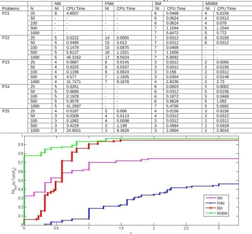
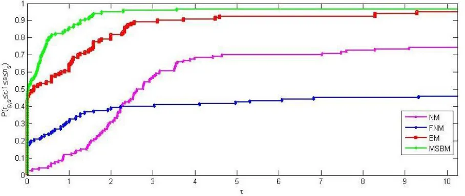
Figure 2. Performance profile of NM, FNM, BM and MSBM methods in term of CPU timeIn the above figures, the left axis of the plot represents the percentage of the test problems for which a method is the best, while the right side corresponds to the percentage of the test problems that were successfully solved by these methods. Figure1 and 2 represent the performances profile in terms of the number of iteration and CPU time (seconds) respectively.
Tables 1−3 and figures 1 and 2 have shown that using the two-step approach in building the Broyden’s updating scheme has significantly enhanced the performance of the classical Broyden method. This observation is glaring when considering CPU time and number of iterations (NI). In addition, it is worth mentioning that the result of MSBM in solving problem7, when the dimension increases, shows that our new approach becomes a better candidate.
5. CONCLUSION
In this paper, we have presented a new method (MSBM) for solving system of nonlinear equations. Unlike the single step, the method employs a two-step to update the non-singular Broyden’s matrix in approximating the Jacobian matrix. Numerical experiments shown strong indication that our new approach requires less computational cost and number of iterations as compared to the NM, FNM and BM methods. Hence, we can wind up that our method (MSBM) is a better candidate when compared with NM, FNM and BM methods in solving system of nonlinear equations.
REFERENCES
[1] C.G. Broyden. A class of methods for solving nonlinear simultaneous equations. Math. Compute. 19:577–593, 1965.
[2] E.D. Dolan and J.J. More. Benchmarking optimization software with performance profiles. Math. Program. Ser, 91:201–213,
2002.
[3] Jr.J.E. Dennis and H. Wolkowicz. Sizingand least-change secant methods. SIAM Journal on Numerical Analysis, 30(5):1291–
1314, 1993.
[4] I.A. Moghrabi J.A.Ford. Multi-step quasi-newton methods for optimization. J. Compute. Appl. Math., 50:305–323, 1994.
[5] I.A. Moghrabi J.A. Ford. Alternating multi-step quasi-newton methods for unconstrained optimization. J. Compute. Appl. Math., 82:105–116, 1997.
[6] S. Tharmlikit J.A. Ford. New implicite updates in multi-step quasi-newton methods for unconstrained optimization. J.Comput. Appl. Math., 152:133–146, 2003.
[7] M. Mamat K. Muhammad and M.Y. Waziri. Abroyden’slike method for solving systems of nonlinear equations. World Applied Aciences Journal, 21:168–173, 2013.
[8] C.T. Kelly. Solving nonlinear equations with Newton’s method. SIAM, 2003.
[9] W.J. Leong M. Faridand M.A.Hassan. Anew two-step gradient-type method for large- scale unconstrained optimization, computers and mathematic switch applications. Computers and Mathematics with Applications, 59(10):3301–3307, 2010.
[10] W.J. Leong M.Y. Waziri and M. Mamat. A two-step matrix-free secant method for solving large-scale systems of nonlinear equations. Journal of Applied Mathematics, doi:10.1155/2012/348654 (Article ID: 348654):9pages, 2012.
51
[12] C.S.Eisenstat R.S.Demboand T Steihaug. Inexact newton method. SIAM JNumer.Anal., 19(2):400–408,1982.[13] J.E. Dennis R.B.Jr. Schnabel. Numerical Methods for Unconstrained Optimization and Nonlinear Equations. Prentice-Hall, Englewood Cliffs, NJ, 1983.
[14] S.WENYU and Y.YUAN. Optimization Theory and Methods. Springer Optimization and Its Applications, 2006.