A Comparative Study of Various Location Prediction and
Interpolation Techniques
J.Ananthi1,*, S.Hamsa Nandhini2, Dr.N.Sengottaiyan3
1Assistant Professor, Department of Computer Science and Engineering, Hindusthan College of Engineering and Technology, Coimbatore,
Tamilnadu, India-641032
2Assistant Professor, Department of CT-PG, Kongu Engineering College, Perundurai, Erode, Tamilnadu India-638060
3Director Academics, Sri Shanmugha College of Engineering and Technology, Pullipalayam, Sankari Taluk, Salem, Tamil Nadu, India-637304
E-Mail: [email protected],[email protected]2, [email protected]3
Abstract
Natural catastrophe is a common phenomenon by which the living as well as nonliving entities belong to the environment faces the calamity. But the human beings can presume the disaster and take major steps to prevent it. There are many technologies available to foresee and prevent the abnormalities or variations in uncovered open regions. Wireless Sensor and Actuator Networks are exploited to monitor the physical and environmental conditions and is preferred due to its cost effectiveness, faster data transfer and accurate computation of required parameter for prediction and prevention. The WSANs are utilizing conditions such as temperature, sound, pressure, location to predict the Geological, Hydrological, and Meteorological disasters. The work mainly aims at studying about the various interpolation techniques and its advantages, disadvantages. The paper finally produces a comparative study of those interpolation techniques and finding an optimal interpolation method for wireless sensor networks.
Keywords: Wireless Sensor Networks, Interpolation techniques, Location Prediction Received on 19 May 2018, accepted on 29 July 2018, published on 12 September 2018
Copyright © 2018 J. Ananthi et al., licensed to EAI. This is an open access article distributed under the terms of the Creative Commons Attribution licence (http://creativecommons.org/licenses/by/3.0/), which permits unlimited use, distribution and reproduction in any medium so long as the original work is properly cited.
3rd International Conference on Green, Intelligent Computing and Communication Systems - ICGICCS 2018, 18.5 - 19.5.2018, Hindusthan College of Engineering and Technology, India
doi: 10.4108/eai.12-9-2018.155741
are frequently used for real time applications such as altitude, rain level of fall and density of chemicals and intensity of
sound and so on. Atmospheric sciences are making use of interpolation methodologies to clearly predict the point values to optimize the progress.
1.2 Spatial correlation
The observations are not independent during the analysis. The spatial correlation is a measure to illustrate the relationship between two close points. Given a set S containing n geographical units, it refers to the relationship between some variable observed in each of the n localities and a measure of geographical proximity defined for all n(n– 1) pairs chosen from S’. Figure 1 represents the sample spatial correlation that illustrates the relationship between group of points.
Figure1. Spatial Correlation
on Energy Web and Information Technologies
Research Article
1. Introduction
A wireless sensor and actuator network connects the number of nodes who are sensing the surface datum from the environment and the actuators acting as servos connected with the sensors as hubs. The sensed data transmission can be autonomous or human controlled. The WSANs were initially developed for the purpose of military and government agencies to monitor their battlefield and the associated environments. Nowadays WSANs are utilized for more number of commercial applications such as monitoring and controlling of industrial settings, telemedicine and scientific development.
1.1 Interpolation techniques
To exclaim values anywhere between two points interpolation techniques are utilized. Interpolation is the course of using fine recognized values to guesstimate unidentified values. A variety of interpolation methodologies
2. Related Works
2.1
Probabilistic
Approach
using
Interpolation
Ioannis C. Paschalidis, Keyong Li, and Dong Guo [1] given a probabilistic approach for identifying or locating the wireless sensor network devices using signal strength measurements called RSSI. The initial localization problem is formed as a hypothesis problem. Appropriate probabilistic descriptors with the position of the devices in the neighboring space are using a pdf interpolation technique. This is done from the measurements between transmitters and receivers on the set of landmarks. From that, the localization system based on the descriptors and the measurements of cluster head in certain landmarks is developed. The requisite theory is developed to characterize the error probability and optimal problem addressing to place clusters and its heads
2.2 MCL Algorithm for Location Prediction
Zhiyu Qiu, Lihong Wu, Peixin Zhang [2] found the idea to satisfy the increase in demand of wireless sensor networks applications in mobile nodes due to technical challenges. This work is constantly focusing on for mobile nodes on location algorithm that continuously focusing on mobile node movement. An improved localization algorithm fully based on Monte Carlo Algorithm is proposed to reduce the interval of sampling points. By considering the stochastic motion model the accuracy of the position is improved using the node’s motion prediction and position filtering. As MCL algorithm is a distributed algorithm it leads to the advantageous for its simple algorithmic structure, strong adaptability and inference level
2.3 Predicting user location using Temporal
Spatial Model
Yantao Jia Yuanzhuo Wang and Xiaolong Jin [3] implemented the prediction of user's locations in social networks that depends on the most prominent associate members of the user, which the majority of the presented location prediction methods fail to attach importance to. It gives a procedure to calculate the maximum accuracy for predicting locations by virtue of the friend’s location. It also proposed the prominent friend selection strategy and narrow down the gap between them and it’s fully based on the influence on the user location. For finding the influential friend’s the temporal spatial Bayesian model is utilized to distinguish the dynamics of friends influence for predicting locations
2.4 Random Walk Based Location Prediction
Approach
Zhaoyan Jin, Dianxi Shi, Quanyuan Wu, and Huining Yan [4] implemented a methodology to overcome the problems faced in localization. The location histories of mobile objects are considered as the matrix for rating and then utilized a random walk based social recommender algorithm for future location prediction process of mobile objects. In addition to that a social slope one recommender method, have been implemented to find slope one suggestions in the rating the
matrix and uses slope one for predicting unknown ratings and it has higher prediction accuracy and lower computational complexity and also it can solve the rating matrix sparsity problem more effectively than previous works.
2.5 Scan Localization System for WSNs
K. Sun, W. Huang, Sachula Meng, Y. Xiao, M. T. Wang, and Z. Xiao [5] executed a novel localization scheme that implements laser beam scan localization and it’s a combination of both grid and light with mobile localization policy. The plan makes use of a moving location assistant (LA) with a laser beam, through which the deployed area is scanned. The Local Assistant sends identities to unknown nodes to obtain the locations of sensor nodes. Through this method high localization accuracy is achieved without the assist of expensive hardware on sensor nodes.
2.6 PSO Based Localization Scheme for
Wireless Sensor Networks
Santar Pal Singh and Subhash Chander Sharma [6] discovered a localization scheme based on the range measurements where the range free methods are considered for cost efficient alternatives. A modified version of DV-Hop called as range free method has been implemented in MATLAB to overcome the positioning error which is named as meta-heuristic (PSO) technique. The performance of the algorithm is analyzed by using the measure localization error and it improved the location accuracy when it’s compared to DV-Hop and improved DV-Hop algorithm (IDV-Hop)
3. Various Interpolation Techniques for
Location Prediction
There are so many interpolation methodologies that can be exploited to predict the new position in an open or closed surface. Interpolation techniques are considered as a constructive technique for optimally identifying the positions mainly focusing on energy efficiency.
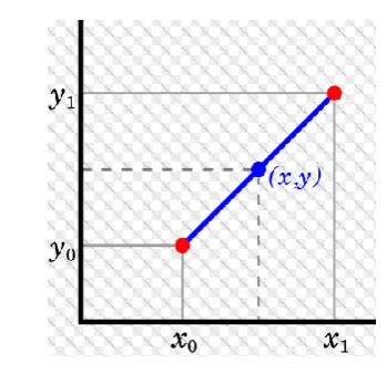
3.1 Linear Interpolation
Figure 2. Linear interpolation
3.2 Cressman Interpolation
The cressman interpolation finds the data for the grid that consists of latitude and longitude grid. So many passes are to be done through grid continuously to increase the precision value of influential radii value. Every pass calculates the new value for the grid using its correction factor. The influential radius value is mentioned as the higher radius from the point of grid to the station. The station beyond the influential radius does not have bearing on the point of grid. The correction factor for cressman interpolation is calculated by analyzing every station which is within the limit of influential radius. An error of a station is described as the variation of the station values and the interpolated value from the grid to the particular station value. Distance weighted formula is applied to the errors that are found within the influential radius level to reach the corrected value of grid point. The correction factor is then used for all grid points before the next pass is done. So the grid point that is nearer will get the most weight. Figure 3 illustrates the cressman interpolation on location prediction based on the cressman weight function given below. If the distance is increased, the total observations are having less weight. The cressman function finds the weight by using the formula below:
W = (RA2 - ra2) / (RA2 + ra2)
Where,
RA - Radius of Influence
ra - Distance between the station & the point.
Figure 3. Cressman Analysis
3.3 Weaver Analysis
Weaver analysis is diverse from the Cressman analysis where a weaver function can be used to perform unweighted interpolation. The observations that are made in the grid box are utilized to calculate the value which is being interpolated. Here the weaver function is not used for calculating the weighed values of observations. Each grid box has the value by calculating an arithmetic average function of the observation. Figure 4 shows the example of Weaver Analysis function which is mainly created for Climate Prediction Center for predicting and analyzing the climate changes
Figure 4. Analysis of Climate changes using weaver analysis
3.4 Inverse Distance Weighted (IDW)
The IDW interpolator always proceeds with the points that are farther away rather than closer one. The points will be either specific or the points in specific radius. This is used to determine the possible output of the location. High variable data makes use of IDW because of easy returning process to collection site and easy to register a new value that are different from original one within the certain area. IDW interpolator implements the assumptions that are closer and alike. IDW uses the values surrounding the prediction location to predict the unmeasured location. The predicted location will be more influential when it is closer. The Figure 5 show the projection and location prediction based on the given input from the open surface area.
3.5 Natural Neighbor Inverse Distance
Weighted (NNIDW)
Interpolation and extrapolation are implemented by NNIDW method. It is facilitated with the cluster of scatter points and manages the input datasets that are large. It is a geometric estimation method which utilizes the neighboring regions around the points in the set of data. This interpolator makes up the exact surface model from the data ser and also it’s very distributed or very linear. Figure 6 shows a sample natural neighbor IDW interpolation method
Figure 6: Natural Neighbour Inverse Distance Weighted Interpolation
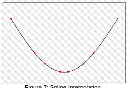
3.6 Spline Interpolation
Spline Interpolation utilizes a mathematical functionality which minimizes the curvature into a smooth surface. It passes through the input points provided. The spline interpolation is made for fixing the mathematical function to the specific nearer input points when the sample points are considered. The spline interpolation is categorized into regularized spline and tension spline. The first method makes a smooth and even changing surface that consists of values lying outer to the given sample range. Three kinds of derivatives considered as slope, rate of change in slope and change in rate of second derivative for calculations. The second method exploits first and second derivatives and it considers many points for calculations aiming to smoother surfaces. So the computational time will be high for this interpolation. Figure 7 represents a natural spline that utilizes a mathematical function to predict the point over smooth surface areas
Figure 7: Spline Interpolation
3.7 Kriging Interpolation
Kriging is a geostatistical interpolation that believes both distance and the variation degrees to estimate the unknown data points [7]. A surface is made based on the points identified using Z-values. The direction of points and the distance depends on the points that are spatially correlated as mentioned in the kriging. Kriging interpolation is an appropriate one when the data is spatially correlated. This interpolation is used in improvisation of soil science and geology. Figure 8 shows the kriging interpolation where the points are predicted based on the distance that are spatially correlated.
Figure 8: Kriging Interpolation
The construction of the kriging interpolation is given based on sum of data as follows:
N
x1
Wx Z(px)
=
Z(p0)
where:
Z(px)= the measured value at the xth location
Wx = an unknown weight for the measured value at the ith
location
p0 = the prediction location
N = the number of measured values
Kriging Interpolation is of few types given below
a.
Ordinary Kriging
Ordinary kriging implements the function F(s) = c + ε(s), where c is an unknown constant. This assumption is rejected for sometimes because ordinary kriging is either using semivariograms or covariances. It also uses transformations which lead to measurement error
b.
Simple Kriging
Simple kriging gives the function as F(s) = c + ε(s), where c is a known constant. Here the Simple kriging can make use of semivariograms or covariances. It also considers transformations that leads to measurement error.
c.
Universal Kriging
d.
Indicator Kriging
Indicator kriging provides the function B(s) = c + ε(s), where c is an unknown constant and B(s) is a binary variable. The binary data is created through some threshold value obtained from continuous data or the observed data from 0 to 1. It is same as ordinary kriging method that either use semi variograms or covariances except the use of binary values.
e.
Probability Kriging
Probability kriging makes the model with B(s) = B(F(s) > ct) = c1 + ε1(s), Z(s) = c2 + ε2(s), where B(s) is a binary
variable created by threshold indicator, B(F(s) > ct) and c1
and c2 are unknown constants. The random error is found on
ε1(s) and ε2(s), for checking autocorrelation for themselves
and cross-correlation between the two errors ε1(s) and ε2(s).
It’s identical to indicator kriging, but exploits cokriging for the betterment of processing. Probability kriging exercises semivariograms or covariances with cross-covariances, and transformations and does not authorize for measurement error.
f.
Disjunctive Kriging
Disjunctive kriging assumption directs to f(F(s)) = c1 + ε(s),
where c1 is an unknown constant and f(F(s)) is an arbitrary
function of F(s). The function f(F(s)) = B(F(s) > ct),for
indicator kriging is a container of disjunctive kriging. To attain disjunctive kriging, a bivariate normality assumption and approximations is needed for the function fi(F(si)) where the assumptions and solutions are difficult to validate. Disjunctive kriging use either semi variograms or covariances with transformations which is not allowing the measurement error.
4. Pros and Cons of Interpolation
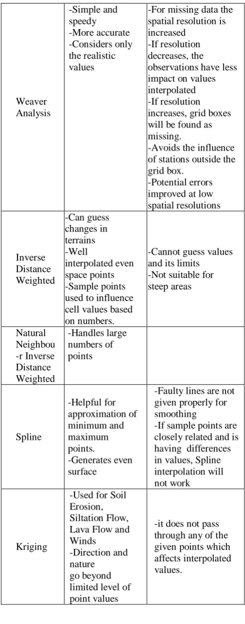
The Table I illustrates the advantages and disadvantages of using various interpolation techniques over location prediction.
Table 1: Pros and Cons of interpolation
Inter po-lation
Advantages Disadvantages
Linear
-The rate of change within a segment is constant
-Discontinuities in derivative exist at all key frame points. Cressm an -easy and computationally speedy -Added accuracy than other methods
-Unstable if density is higher than station density
-Sensitive to errors observed
-Analysis gives the unrealistic extreme grid values,
-Does not consider the distribution of observations related to each other. -Consistent results varies with observed one
Weaver Analysis -Simple and speedy -More accurate -Considers only the realistic values
-For missing data the spatial resolution is increased
-If resolution decreases, the observations have less impact on values interpolated -If resolution increases, grid boxes will be found as missing.
-Avoids the influence of stations outside the grid box.
-Potential errors improved at low spatial resolutions Inverse Distance Weighted -Can guess changes in terrains -Well interpolated even space points -Sample points used to influence cell values based on numbers.
-Cannot guess values and its limits -Not suitable for steep areas Natural Neighbou -r Inverse Distance Weighted -Handles large numbers of points Spline -Helpful for approximation of minimum and maximum points. -Generates even surface
-Faulty lines are not given properly for smoothing
-If sample points are closely related and is having differences in values, Spline interpolation will not work
Kriging
-Used for Soil Erosion, Siltation Flow, Lava Flow and Winds -Direction and nature go beyond limited level of point values
5. Conclusion
In this paper the fundamental concepts of wireless sensor networks have been discussed and the various common phenomenon identification methodologies are discussed. The introduction is about spatial correlation, the interpolation technique and the use of interpolation in identifying the new points on an open surface area. Various models have been implemented for localization of sensors such as probabilistic approach, MCL algorithm, Random walk based algorithm, Temporal Spatial model, PSO based model and Scan localization System etc. for predicting a point for sensor localization. The localization is mainly focusing on the network optimization in terms of cost and energy efficiency. To overcome the previous implementations the interpolation techniques are implemented. This is fully based on the prediction of new surface points if the points are already predicted and given as an input. The paper is discussed for various techniques for sensor localization and various interpolation methods for variety of prediction methods used by various applications in sensor networks through its advantages and disadvantages.
6. References
[1] Dong Guo, Ioannis C. Paschalidis and Keyong Li, “Model-Free Probabilistic Localization of Wireless Sensor Network Nodes in Indoor Environments”, Springer-Verlag Berlin Heidelberg, pp. 66–78, 2009.
[2] Zhiyu Qiu, Lihong Wu and Peixin Zhang, “An Efficient Localization Method for Mobile Nodes in Wireless Sensor Networks”, International Journal of Online Engineering (iJOE), Vol. 13, No. 3, 2017.
[3] Xiaolong Jin, Xueqi Cheng, Yantao Jia and Yuanzhuo Wang, “TSBM: The Temporal-Spatial Bayesian Model for Location Prediction in Social Networks”,IEEE/WIC/ACM International Joint Conferences on Web Intelligence (WI) and Intelligent Agent Technologies (IAT), 2014.
[4]Dianxi Shi, Huining Yan,QuanyuanWu, and Zhaoyan Jin, “Random Walk Based Location Prediction in
Wireless Sensor Networks”, International Journal of Distributed Sensor Networks, Vol. 9 Issue 12, 2013.
[5] W. Huang, K. Sun, Sachula Meng, M. T. Wang, Y. Xiao and Z. Xiao, “Implementation of a novel scan localization system for wireless sensor networks”, Journal of Laser Applications, Vol 25, Issue 1,2013.
[6] Santar Pal Singh and Subhash Chander Sharma, “Implementation of a PSO Based Improved Localization Algorithm for Wireless Sensor Networks”, IETE Journal of Research, 2018.