R E S E A R C H
Open Access
Unpaved road detection based on spatial
fuzzy clustering algorithm
Jining Bao
1, Yunzhou Zhang
2*, Xiaolin Su
1and Rui Zheng
1Abstract
Vision-based unpaved road detection is a challenging task due to the complex nature scene. In this paper, a novel algorithm is proposed to improve the accuracy and robustness of unpaved road detection and boundary extraction with low computational costs. The novelties of this paper are as follows: (1) We use a normal distribution with infrared images to detect the vanishing line, and a trapezoid prediction model is proposed according to the road shape features. (2) Road recognition based on connected regions is implemented by an improved support vector machine (SVM) classifier with a normalized class feature vector. According to the recognition results, the road probability confidence map is obtained. (3) With the help of fusing continuous information with the trapezoidal forecasting model and the probability from the confidence map, we present a road probability recognition method based on the trapezoidal forecasting model and spatial fuzzy clustering. Furthermore, the histogram backprojection model is used to solve interference problems caused by shadows on the road. It takes approximately 0.012~0.014 s to process one frame of an image for the road recognition, and the accuracy rate can reach 93.2%. The
experimental results show that the algorithm can achieve better performance than some state-of-the-art methods in terms of detection accuracy and speed.
Keywords:Unpaved road detection, Confidence map, Trapezoid prediction, Vanishing line detection, Clustering analysis
1 Introduction
The intelligent vehicle remains a core problem in com-puter vision technology and has numerous potential ap-plications, such as driver assistance, transportation system scheduling, and searching for the optimum route. There is no doubt that road detection has become one of the most popular topics in computer vision [1–3]. Computer vision technology is very suitable for road de-tection since it includes a large amount of dede-tection in-formation and accurate sensing [4, 5]. However, road detection is still challenging due to different road types and various background, weather, and illumination conditions.
Over the past few decades, numerous approaches have been developed for road detection. According to the structuralization degree, existing road detections can be classified into two categories: paved road detection and
unpaved road detection [6]. For the well-paved roads with remarkable road borders and lane markings, desir-able road detection accuracy can be achieved by many existing methods. However, unpaved roads are most commonly seen in suburban, rural, and battlefield envi-ronments. Since there are hardly any variant features to characterize unpaved roads [7,8], it is challenging to de-velop a valid algorithm with computer vision. Obtaining accurate road information under unfavorable interfer-ences plays a critical role in unpaved road detection [9]. The main difficulty in unpaved road detection based on computer vision is that the detection algorithm must be able to handle complex and unknown scenes, such as road types with variable illumination, different weather conditions, and varieties of textural characteristics. Fur-thermore, intelligent transportation systems generally re-quire fast processing since the vehicle speed is bounded by the processing rate [10]. All of these factors impact the unpaved road detection results.
Some algorithms have been proposed for road detec-tion by researchers. The algorithms can be mainly * Correspondence:[email protected]
2Faculty of Robot Science and Engineering, Northeastern University,
Shenyang 110819, China
Full list of author information is available at the end of the article
divided into three categories: feature-based, model-based, and ML (machine learning)-based [11–13]. Algo-rithms based on features usually extract significant and stable features. These algorithms are very simple and rapid. For example, color features [14] are often applied to extract the road region from an image. However, they do not work well for general road images, especially when the roads have little color differences between their surface and the environment. The traditional feature-based algorithm is not suitable for complicated scenes since it is insensitive to road shapes and is easily impacted by watermarks, shadows, vehicles, and pedes-trians. A series of features are analyzed to show their ability to detect road surface from background. There-fore, it is often combined with other algorithms for seg-mentation processing to obtain proper features. The top-down road recognition algorithm [15] combines both the region and boundary cues of the images. With an off-line classifier, it can detect road regions. Shang et al. [16] proposed an approach to find a way to choose the feature descriptors. Meanwhile, support vector ma-chine (SVM) technology has been added to analyze the importance of the common feature descriptors during the road detection process. Compared with the feature-based algorithm, the model-feature-based algorithm matches the mathematical model according to the prior information, such as the road position, distribution, and shape. Kluge et al. [17] proposed a deformable template model of lane structures to locate lane boundaries without threshold-ing the intensity gradient information. The Metropolis algorithm is used to maximize a function that evaluates how well the image gradient data support a given set of template deformation parameters. The multi-modal road detection and segmentation algorithm [18] is proposed based on monocular images and HD (high definition) multi-layer lidar data (3D point cloud). The detection al-gorithm for road boundaries is proposed by using the hyperbolic road model for moving images captured by in-vehicle cameras [19]. This algorithm uses the detected center lines based on edges for parameter estimation, and only the region of validity of the detection result of the center line is applied in the hyperbolic road model. These algorithms have strict demands on the shape of the road region and require precise mathematical models. At present, this type of algorithm is mainly used for simple road detection. The ML-based algorithm needs to collect a large number of samples and training parameters. Typically, SVM-based algorithm is applied to road detection through semi-supervised or supervised online learning [20, 21]. For example, Zhou et al. [22] proposed an effective approach to use SVM for road de-tection with self-supervised online learning. Yun et al. [23] adopted the boosting, SVM, and random forest clas-sifiers to evaluate the correlation feature set and raw
feature set. To fully utilize potential region feature corre-lations and improve the classification accuracy, this algo-rithm also introduces the feature combination method into road detection. K-means algorithm and density-based spatial clustering of applications with noise (DBSCAN) algorithms are also significant means of clus-tering road regions [24, 25]. Road detection is also im-plemented using a neural network [26]. Although it can achieve high accuracy, its performance often depends on the large amount of training data and complex computations.
The vanishing line is an important component in road detection. With the aid of a set of prior information, road detection is improved. The vanishing line is located horizontally between the road and sky. The upper part is the sky and the lower part is the road in general. The distribution characteristics of the road region assist in segmenting the road region to reduce the error rate of vanishing line detection. Most common methods, such as Prewitt, Sobel, and Gabor filters, detect the vanishing line [27]. To date, many algorithms have attempted to handle off-road conditions. These algorithms have their own advantages and disadvantages. Compared with the significant advances in paved road detection, little pro-gress has been made for unpaved roads [10,15].
When a vehicle is driven on an unpaved road, illumin-ation variillumin-ation easily leads to a poor visual condition, which makes it difficult for the driver to distinguish the unpaved road. Compared with the paved road, there is still a large space for improvement in unpaved road de-tection. First, with respect to road textures, unpaved roads mostly have poor conditions, such as shadows and ruts. Second, the road boundary is fuzzy and difficult to identify. Sometimes the ruts are more obvious than the road boundary. Last, there are some variable factors, such as varying illumination and changing weather con-ditions. It is significant to propose a good performing al-gorithm using computer vision for practical applications of unpaved road [10]. Therefore, we propose a new, more efficient method for unpaved road detection based on infrared images in this paper.
interest (ROI) is obtained, and the trapezoid mode is established. (2) An improved SVM classifier is constructed based on the unidentified connected region, and a road probability confidence map is also generated according to the recognition results. (3) The road region is determined by the spatial fuzzy clustering algorithm. The fuzzy C-means (FCM) algorithm that combined with the trapez-oidal forecasting model and the probability confidence map is adopted to improve the accuracy of road boundary detection. Meanwhile, gray-based histogram backprojec-tion compensates for the missing parts after road cluster-ing due to segmentation and other reasons. Therefore, we can obtain more accurate boundary information.
The remainder of this paper is organized as follows. The proposed algorithm is detailed in Section2. Section
3 presents the experimental results and a discussion of the proposed algorithm. Finally, Section 4 draws some conclusions for the paper.
2 Methods
In this section, we detail the proposed FCM-based un-paved road detection framework. It is designed with the following steps: (1) vanishing line detection based on the normal distribution with infrared images; (2) an image segmentation method that uses the double-Otsu algo-rithm and the trapezoid prediction is obtained; (3) image classification with the improved SVM and construction of the probability confidence map according to the classifica-tion results; (4) spatial fuzzy clustering algorithm based on FCM combined with the trapezoidal forecasting model and the probability confidence map to complete road rec-ognition; and (5) grayscale-based histogram backprojec-tion to weaken the interference caused by road shadows.
2.1 Vanishing line detection
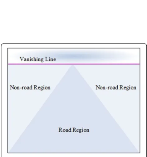
Normally, an unpaved road boundary is blurry and diffi-cult to recognize. Real-time image information should be utilized as much as possible to improve the detection accuracy. Real-time video collected by an infrared imager contains substantial prior information: (1) the road presents fixed geometrical features, such as trian-gles or trapezoid; (2) the upper region of the infrared image is the sky, the middle area is the road, and both sides are mostly non-road areas; and (3) consecutive frames of infrared images present spatio-temporal con-tinuity. The road changes are relatively continuous and stable without abrupt changes. The position of the road region in the next frame can be predicted based on the image information in the previous frame.
2.1.1 Image pre-processing
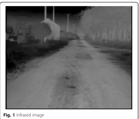
Images captured by a vehicle-mounted infrared imager have 702 × 576 pixels, as shown in Fig. 1. By removing
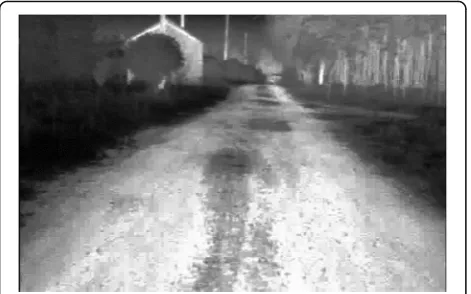
the worthless border, the image is resized to 696 × 450 pixels to obtain the ROI. Based on image pre-processing, the original infrared image can remove noise to enhance the contrast and weaken the inference in the image. After histogram equalization, the infrared image is shown in Fig.2. The detailed boundaries of the road are enhanced without affecting the overall contrast of the entire image.
2.1.2 Vanishing line detection
Vanishing line detection can remove irrelevant areas over the horizon to reduce computations and improve accuracy. As the juncture area of the sky and the road area, the vanishing line always appears as a longer line. Furthermore, it has an obvious vertical gradient.
In this paper, the vanishing line detection and tracking method based on the normal distribution is proposed according to the estimate of the vanishing line. Bayesian posterior is used to detect the vanishing line with a priori probability that obeys the normal distribution. When the current frame detects the vertical gradient feature, the probability at positionhmis:
p hmð Þtlið Þt
¼p li
t
ð Þ h
mð Þt
p hmhmðt−1Þ
p lð Þit
ð1Þ
where p(hm(t)|li(t)) is the probability of the vanishing line at the positionhmwhen the current frame detects vertical gra-dient feature. The vertical gragra-dient feature is the probability of vanishing line denoted by p(li(t)|hm(t)). p(hm(t)|hm(t−1)) is a priori probability, that is, the current frame probability is predicted from the last frame normal distribution. pðlðtÞi Þ
denotes theith linearlin vanishing line probability.
p lið Þt jh
¼p lið Þt h1ðt−1Þ
p h1ð Þthmðt−1Þ
þp lið Þth2ðt−1Þ
p h2ð Þt hmðt−1Þ
þ⋯þp lið Þthnðt−1Þ
p h1ð Þt hnðt−1Þ
ð2Þ
where pðlðtÞi jhÞ is a constant to all of the image frames.
Bayesian posterior probability can be calculated with the aim of accurately localizing the vanishing line.
2.2 Segmentation method
2.2.1 Double-threshold segmentation based on the Otsu method
As one of the most effective and widely used methods [28,29], Otsu threshold method is adopted for road seg-mentation. It selects a threshold using the histogram of a grayscale image to find the image’s optimal threshold, which maximizes the inter-class variance to obtain a lar-ger separation between the foreground and background. Moreover, it has low computation complexity, which is suitable for a real-time system. Given an image I that containsNpixels and gray levels ranging from 0 tom− 1, there arenipixels for gray leveliand its probability is pi:
pi¼ni=N ð3Þ
N¼X
m−1 i¼0
ni ð4Þ
We set the threshold as t, the ratio of the number of pixels in the ROI to the entire image area is denoted asω0(t), and the mean grayscale value of the target
re-gion isμ0(t). The ratio of the pixels in the non-target
re-gion to the entire image isω1(t), and the mean of
non-target region isμ1(t).We obtain the following equations:
ω0ð Þ ¼t
X
0≤i≤t
p ið Þ
μ0ð Þ ¼t
X
0≤i≤t
ip ið Þ=ω0ð Þt
8 > < >
: ð5Þ
ω1ð Þ ¼t
X
0≤i≤m−1
p ið Þ
μ1ð Þ ¼t
X
0≤i≤m−1
ip ið Þ=ω1ð Þt
8 > < >
: ð6Þ
Average grayscale value of the entire image can be expressed as:
μ¼ω0ð Þt μ0ð Þ þt ω1ð Þt μ1ð Þt ð7Þ
The inter-class variance valueϑ:
ϑ¼ω0ð Þt ðμ0ð Þt −μÞ 2þω
1ð Þt ðμ1ð Þt −μÞ
2 ð
8Þ
We choose T as the optimal segmentation threshold whenϑ achieves the maximum value using the traversal method.
Otsu threshold segmentation can effectively extract the road region. However, the intensity between the road and surrounding scenery is always small, which causes poor segmentation results. Furthermore, the shadows are closer to the non-road region. Therefore, threshold segmentation can only be used for the initial classifica-tion. To solve this problem, we proposed a double-Otsu threshold segmentation method. For the initial segmen-tation, Otsu method was used to obtain the threshold T1.Then, it is used again to segment the image over the T1~255 range to achieve the second threshold T2. After
that, two segmentation images can be obtained by thresholdsT1andT2.
Accordingly, the thresholds ranging from 0 to T1are
chosen for the same operation. We obtain the third seg-mentation threshold T3, which ranges from 0 to T1.
Then,T3is utilized to continue with the threshold of the
segmented image. Meanwhile, the image is divided into blocks using the boundary auxiliary information. Figure3
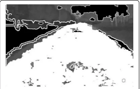
Fig. 3Segmentation map based on double-Otsu method
shows the results of the double-Otsu method. In Fig.3, the white region represents the unknown region, the middle black region denotes the road, and the left black region represents the non-road. The obtained result is better than that of one-time Otsu, which can be used to recognize the road region from the non-road region. The obtained segmentation results provide a foundation for further research.
2.2.2 Trapezoidal forecasting model
Since the road region appears to have a trapezoidal geo-metric shape, there are some correlations between two adjacent frames that will not change in the video [30]. Therefore, the current frame can be used to predict the next frame. The trapezoidal forecasting model is pro-posed based on the characterization of the positional distribution.
Trapezoidal forecasting model can be established with the following steps: (1) To form a trapezoidal image, as shown in Fig. 4a, b, for road prediction in the next frame, four vertices are extracted from the previous frame of the road region and give the value range. (2) Based on the distance parameter of the trapezoidal fore-casting model, the obtained trapezoidal region can be used to determine whether the initial segmentation re-sult is a road region. If the computed distance is far from a certain value, the connected region is assumed to be a non-road region. Otherwise, it is a road region. (3) To extract the road area map as shown in Fig. 4c, we first use the morphological erosion operation with a 3 × 3 disk-shaped structural element to estimate the back-ground of the trapezoid vertex image (see Fig.4b). Then,
the road boundary result (see Fig. 4d) can be obtained by subtracting the background image from the original trapezoidal vertex image. As shown in Fig.4c, d, the re-sults of boundary recognition are relatively accurate. The advantage of this method is that it can cut off the non-road region that is similar to the road region, such as a trunk. However, trapezoidal forecasting model can-not independently achieve excellent results.
2.3 Classification method
ML is often used for road recognition. As a supervised learning technique, SVM selects an optimal hyper-plane as a decision function. Taking into account the empirical error and the complexity of the classifier, SVM is widely used because it can optimize the road boundary [31–33]. Considering the complex recognition tasks, SVM is used to classify road regions in this paper.
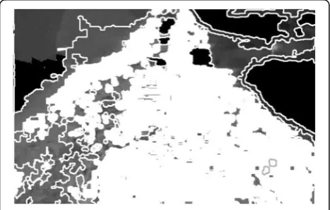
The training results are shown in Fig.5. The white gions are considered to be road regions, the black re-gions are non-road rere-gions, and the other rere-gions are undefined parts of undetected connected areas. The error rates of the trained classifier and positive sample are 7.52 and 1.08%, respectively. In Fig. 5, the road re-gion has large shadow areas and some of it is cut off. Some parts of the road region in the image are unidentified.
2.3.1 Improved SVM classifier
For the SVM classifier, this paper presents two improved methods: feature classification normalization and SVM combination classifier.
Normalization method is adopted to normalize three types of features (grayscale, position, and shape) in the fusion process. This method can retain the dynamic range of the features and affect the training results, but it does not take into account the relationship among several features and each feature within one type of fea-ture. Therefore, we propose three features for classifica-tion and normalizaclassifica-tion. There are a total of 1314 samples, including 467 positive samples (with 413 sam-ples of road regions and 54 road shadows) and 467 nega-tive samples (with 0, 5, and 462 samples of the sky regions, the surrounding trees, and the non-road region, respectively).
Figure 6 shows the classification result of classification-normalized SVM. The obtained result is more accurate and the road region is completely recog-nized compared with Fig.5. The error rate of the trained classifier is 6.79% and the positive sample is 6.79%. The testing time is between 0.003 and 0.006 s. Although the classification normalization loses some of the details of the image, it can retain the independence of each feature and weaken the interference among the three features caused by the fusion.
The SVM combination classifier separately trains three types of feature information, and each piece of informa-tion forms the non-classificainforma-tion normalizainforma-tion and clas-sification normalization features. Therefore, six SVM classifiers are formed depending on the two classifiers and three features’information. Then, we obtain a better SVM classifier through the given weight parameters after the training.
First, the feature information of grayscale, position, and shape are collected. Then, the three features’ infor-mation and one classifier regarded as the base classifier are constructed. We choose one group with the lowest training error rate in each base classifier as the training set, which can be used to obtain SVM classifier. The ini-tial weight of the base classifier is given with the corre-sponding parameter calculated as follows:
ccwnew¼αccwoldþð1−αÞ ccw
pcwnew¼αpcwoldþð1−αÞ pcw
acwnew¼αacwoldþð1−αÞ acw
cnwnew¼αcnwoldþð1−αÞ cnw
pnwnew¼αpnwoldþð1−αÞ pnw
anwnew¼αanwoldþð1−αÞ anw
8 > > > > > < > > > > > :
ð9Þ
whereccwnew,pcwnew,acwnew,cnwnew,pnwnew, andanwnew,
respectively, represent as the training weights of the base classifier in grayscale information non-classification, lo-cation information non-classification, shape non-classification, grayscale information non-classification, loca-tion informaloca-tion classificaloca-tion, and shape informaloca-tion classification. ccwold, pcwold, acwold, cnwold, pnwold, and
anwold, respectively, represent the last corresponding training weight of the base classifier. The last confidence measure is denoted as α= 0.5. ccw, pcw, acw, cnw, pnw, and anw denote the calculated weights in this group. The formula is given as:
ccw¼nccr−ncce
total
pcw¼
npcr−npce
total
acw¼nacr−nace
total
cnw¼ncnr−ncne
total
pnw¼
npnr−npne
total
anw¼nanr−nane
total 8 > > > > > > > > > > > > > < > > > > > > > > > > > > > :
ð10Þ
where nccr, ncce, ncnr, ncne, npcr, npce, npnr, npne, nacr,
nace,nanr, andnane,respectively, represent the base
clas-sifier that predicts the correct or wrong numbers of the normalization of non-classification and classification grayscale information, location information, and shape information in this group. Their summation is calculated as follows:
Fig. 5SVM classification result
total¼nccr−ncceþnpcr−npceþnacr−nace
þncnr−ncneþnpnr−npneþnanr−nane ð11Þ
The parameters and the training results of six base classifiers are shown in Table 1. The added contents are the parametercdenotes penalty factor andσ2represents the kernel function parameter. Each base classifier uses its own penalty factor and kernel function parameters. The training time is 587 s, and the highest support vec-tor tree is 100%. The final discriminant is as follows:
SVM¼ccwSVMccþpcwSVMcpþacwSVMca
þcnwSVMncþpnwSVMnpþanwSVMna
ð12Þ
After training, we get the weight parameters of each classifier: ccw= 0.1347, pnw= 0.2486, anw= 0.347, ccw=
0.1100,pnw= 0.2544, andanw= 0.1176. The error rate of
the combined SVM classifier is 5.04%; the positive sam-ple error rate is 2.05%, and the testing time is between 0.011 and 0.025 s. The result is shown in Fig.7.
2.3.2 Construction of a probability confidence map
A confidence map is established according to the results of SVM discriminant connected area. We set the confi-dence values as 0 and 1 to represent the non-road region and road region, respectively. The formula of the prob-ability confidence is as follows:
p¼
1
f xð Þ=2þ0:5 0
f xð Þ≥1 −1<f xð Þ<1
f xð Þ≤−1
8 <
: ð13Þ
The probability confidence map is converted into a visual image. The conversion formula is calculated as:
Ið Þi;j ¼256p ð14Þ
There is an unrecognized background region in the image that has not been subjected to SVM discriminant, except for the connected region. Given that the result of SVM discriminant is 0, the probability confidence is 0.5 which cannot identify road region or not. The grayscale value is 127 in the probability confidence map.
The converted probability confidence map is shown in Fig.8. (1) In the first group (Fig.8a, b), the road region and road shadow region are marked as white and near white, respectively. This represents the shadow region belonging to the road region based on the SVM method. (2) In the second group (Fig.8c, d), the road region and road boundary region are marked as white and near white, respectively. The non-road region is on the right side of the image and is marked as black. The grayscale value of the gray region on the top and left side of the image is smaller than 127. With the substantial color of probability confidence map, SVM method can correctly discriminate the road region from the non-road region. (3) In the last group (Fig. 8e, f ), the white region repre-sents the road region, while the other connected regions are marked as black except for the non-discriminated re-gions. The probability confidence map shows that the connected region is related to the road region, with a more robust stability and fault tolerance.
2.4 Clustering method
We propose to use Otsu method to obtain connected re-gions and regard each of them as a data point, which can greatly reduce the size of the data set and computa-tional complexity. However, the data points will be sparser and the number of outliers will be increased due to the reduction of data sets. It is crucial to select proper initial parameters and features. The road region is gener-ally in the lower middle image with a relatively stable grayscale value.
Table 1Training results of six basic classifiers on penalty factorcand kernel function parameterσ2
Adopted normalized feature c σ2 Training time (s) Number of positive samples Accuracy (%)
Gray feature (non-classification) 4 256 587 1027 82.9
Location feature (non-classification) 8 8 309 518 41.4
Shape feature (non-classification) 8 512 291 538 43.0
Gray feature (classification) 8 1 291 1314 100.0
Location feature (classification) 8 1 271 1314 100.0
Shape feature (classification) 4 1 339 1144 87.1
It is reasonable to divide the road into three categor-ies, as shown in Fig.9, which are the ideally segmented road regions. The selection of the initialization has a very significant influence on the performance and results of the clustering analysis. The initialed cluster centers are usually several points that are randomly selected from the given data set or the position of a peak of the histogram. In this paper, the size of the processed data set is relatively small, and therefore, it easily generates empty clusters. The road region clustering problem can be solved by the prototype clustering model. FCM clus-tering is one of the prototype clusclus-tering methods.
2.4.1 Road identification based on FCM algorithm and trapezoidal forecasting model
There are many methods for fuzzy clustering [34, 35], and FCM clustering is adopted in this paper.X= {x1,x2,
...,xm} is defined as a dataset that containskclustersC1, C2,..., Ck. wij is a membership value that indicates that
the ability ofxibelongs to Cj, and the sum of the
mem-bership values wijfor a given pointxiis 1.X= {x1,x2, ..., xm} represents the input data point set in FCM
Fig. 8Probability confidence maps.aOriginal image 1#.bProbability confidence map1#.cOriginal image 2#.dProbability confidence map 2#.
eOriginal image 3#.fProbability confidence map3#
algorithm, the number of clusters is C, and the output membership value isw.
In this paper, the points are [x,y,k∗m,d∗t], where x and yare the central row and column coordinates of the connected regions, respectively. k denotes the propor-tional coefficient of the grayscale and the posipropor-tional
infor-mation is k¼
ffiffiffiffiffiffiffiffiffiffiffiffiffiffiffiffiffiffiffiffiffiffi
height2þwidth2 p
256 . m is the gray scale mean value of the connected regions.ddenotes the proportional coefficient of the predictive value and the spatial location information.tis the prediction features. Second, the clus-ters are separated into three categories and the membership matrix is initialized. When the membership matrix is ini-tialized, we select the virtual center in advance. The center point is defined as:[110, 100,k∗thres,d∗t], [110, 596,k∗ thres,d∗t], [255, 348,k∗thres,d∗t], where the predictive parameter valuedis set as 100 andk= 3.24 by height = 450 and width = 696. Then, the initialized membership matrix is calculated. Finally, the parameter value of pis set to 2. The above clustering procedure can be found in [36]. After the calculation, the connected region is sorted into the highest membership degree.
2.4.2 Road probability determination based on FCM algorithm and trapezoidal forecasting model
A single continuity prediction or a single discriminant is prone to generate errors. When the probability confi-dence map is used as the prediction model, the accuracy of SVM classifier cannot achieve 100%. Although FCM clustering algorithm can reduce the error rate of SVM algorithm, the efficiency improvement is limited. The probability confidence map only addresses each frame image and usually neglects the important characteristic of video continuity in the video.
There are still some problems that occur by only using the trapezoidal forecasting model. For example, if the ve-hicles’speed increases too fast, the road continuity will be difficult to maintain in some situations, especially in excessively fast turns. In this case, the continuity of the road is greatly influenced by the concentration of traffic. As shown in Fig. 10, some parts of the road region are not recognized by the trapezoidal forecasting model when the road changes rapidly. Moreover, there are some errors in the identification of the road boundary. The combination of the two types of forecasting infor-mation is proposed in this paper.
The results from FCM clustering algorithm belong to class membership. Based on the characteristics of FCM re-sults, we propose a discriminant correction model, which is based on FCM algorithm and trapezoidal forecasting model of road probability decision model. After the FCM iteration is finished, the connected region of the largest membership class can be regarded as a preliminary result. Furthermore, the membership degree is recalculated by using the mem-bership probability-based confidence map. Finally, a class of connected regions can be selected by means of the max-imum degree of the membership class. The probability con-fidence map represents the probability of the road region. In this paper, FCM is divided into three categories. The first category is the road region, and the other two categories belong to the non-road region. The recalculated member-ship formula is as follows:
Fig. 10FCM clustering result based on trapezoid prediction model
Fig. 11FCM clustering road boundary recognition result based on probability confidence map
wnew¼ w
p; maxð Þw∈c 1
wð1−pÞ; maxð Þw∉c1
ð15Þ
where c1 denotes the first class, w is the membership
after the stopping iteration, and wnew is the final mem-bership of the connectivity region. p is the probability confidence for this connected region, and max(w) is the category of the maximum membership. With the im-proved method, road region identification and road boundary recognition obtain higher accuracy.
Compared with Fig. 10, for the same video frame, Fig. 11 shows a more accurate road recognition result that agrees with the actual environment.
2.4.3 Road recognition based on histogram backprojection method
We consider that the above-mentioned algorithms are all based on connected regions. However, they may lead to incomplete recognition of the road boundary in the following three cases:
1. There are undetected connected regions in the video.
2. Morphological erosion is used to segment the connected region, which reduces the undetected regions as well as reduces the road regions.
3. The non-road connected region is too large or too small, which results in inaccurate road regions.
The histogram backprojection method of the road re-gion model can solve the above-mentioned problems. This method, which is based on pixels, effectively com-pensates for the drawbacks and disadvantages of the connected region as a basic unit.
The histogram backprojection method converts the color histogram of the original image into a color prob-ability distribution. The pixel grayscale value of the ori-ginal infrared image represents the image intensity. The pixels in the probability map are used to recognize the connected regions to determine the real road region. Figure12shows the effect of histogram backprojection.
Although the result of FCM clustering is good, it is not precise enough to use the connected region as the basic unit to recognize the road region. In this paper, the pixel grayscale value of the histogram is used to com-pensate for the missed road parts using histogram back-projection method. First, the histogram is formed by the statistical distribution of the pixel values in the recog-nized road region. Then, the brightness of the histogram peak at the corresponding point is calculated, which re-serves the grayscale 0.8 to 1.2 times. Histogram is cut off as the probability density curve of the road. The entire
Fig. 14Road region marking diagram Fig. 15Road region based on backprojection probability map
image is transformed into a histogram backprojection probability map. The histogram backprojection probability of the image transformed by FCM cluster for the road’s gray-based model is shown in Fig.13.
On the basis of the histogram backprojection, the road regions and road edges are obtained by combining the results of the road region recognition based on the prob-ability confidence of FCM with the trapezoid prediction model. Road region recognition is complemented by the histogram backprojection. This process involves the fol-lowing steps: (1) The boundary of the auxiliary backpro-jection probability map is used to segment the image, while the top region of the vanishing line is removed. (2) Road region recognition based on FCM and the prob-ability confidence map of the trapezoid prediction model is marked by white pixels (255). From Fig.14, it can be seen that the white area (compared with the real road region) is missing. (3) Whether to keep or delete the connected region depends on the presence of the white mark in the residual connected region of the statistical backprojection probability map.
The new road region is used to recognize the road boundary, and the corresponding recognition result is shown in Fig.15. It observed that the road boundary is more accurate and accordant with the characteristics of human vision. The histogram backprojection method based on grayscale values has a good effect on road re-gion recognition, which compensates for the deficiency of the connected region.
2.5 Implementation
The system is implemented on a PC (Intel Core i5 at 3.30 GHz with 16 G RAM). The average running time of every image frame is evaluated with Matlab R2015a on Windows 7. The system is tested under complex field conditions for vanishing line detection, image segmenta-tion, and clustering. Grayscale histogram with infrared images is used for feature correspondence. We deliber-ately selected video clips that were recorded under diffi-cult conditions. All of the images used in our experiment are downloaded from a vehicle-mounted in-frared imager.
3 Results and discussion
In this section, first, we describe the experimental set-ting, including the sample collection, the parameters, and classifier choice. Then, the comparison of the van-ishing line detection results is depicted. Finally, we com-pare the proposed approach with the state-of-the-art approaches in terms of accuracy and time consumption. Fig. 16Samples after labeling
Fig. 17Error rate with different Rbf parameters
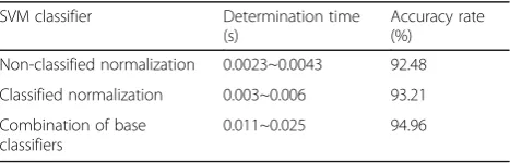
Table 2Performance comparison of three SVM classifiers
SVM classifier Determination time (s)
Accuracy rate (%)
Non-classified normalization 0.0023~0.0043 92.48
Classified normalization 0.003~0.006 93.21
Combination of base classifiers
3.1 The experimental setting 3.1.1 Sample collection
Three features (grayscale, position, and shape) are used as the extracted features. Although there is no RGB (red, green and blue) color information, the infrared image can provide plenty of information in grayscale. Grayscale frames in the road region are different according to changes in the road conditions, but the grayscale distri-bution in a continuous video is stable. Furthermore, the grayscale value of the road shadow is lower than that of the road region, where the background is on both sides of the road in the image. In a relatively simple scene, lo-cation information can also provide a priori information which is very important in road recognition. For ex-ample, the road is at the bottom and the middle of the image, while the sky is at the top. In addition, we adopt the shape features due to the meaningful connected re-gions extracted in our paper.
In this section, extensive experiments are discussed that were used to validate the effectiveness of the pro-posed approach on a private image database from a Chinese military project. The infrared images captured by the vehicle-mounted infrared imager have a fixed 702 × 576 resolution with the D1 format. We marked 93 images that were selected from the vehicle-mounted in-frared video in natural fields. These selected images con-tain road bends, forks, and shadows, which are used to validate the effectiveness of the proposed approach by
comparing the results with the ground truth. The recur-ring objects in the images roughly contain roads, shadows, sky, surrounding trees, and other non-road re-gions of unknown materials. The marked results are shown in Fig. 16: white (255) represents the road, and black (0) represents the shadowed parts of the road. The sky is marked as 180, the non-road and unknown re-gions are marked as 120, and the trees are marked as 60. Then, we extracted features from the marked images to generate a total of 1854 samples. Among them, there are 826 road samples and 94 road shadow samples, totaling 920 positive samples. Furthermore, there are 934 nega-tive samples with 0, 10, and 924 samples of the sky re-gions, surrounding trees and non-road regions, respectively. Ten-fold cross-validation is adopted to se-lect the smallest error as the training set.
3.1.2 Parameter setting
Radial basis function (Rbf ) kernel is chosen and the ker-nel function parameterσ2and penalty factorcare deter-mined by the grid method. There are 25 different groups. σ2 takes [2-2,2-1,20,21,22], and c takes [21,22,23,24,Inf]. We chose the minimum error rate group as the selected parameter in the groups. The number of training samples is reduced to 102 to save time. The classification performance of different parameters is shown in Fig.17. It can be seen that the error rate is the Fig. 18Vanishing line detection.aVertical gradient map based on Sobel operator.bVanishing line detection result
smallest when setting σ2= 1 and C= 8 are used as the parameters for the training set.
3.1.3 Classifier selection
In this paper, we proposed three SVM classifiers: the non-classified normalization classifier, classified normalization classifier, and combination classifier with the above two classifiers, as shown in Table2. Although the accuracy of the combined classifier is high compared with the other two methods, the discriminant procedure is time-consuming. The accuracy of the classification normalization classifier is relatively higher compared with that of the non-classification one, and the add-itional time is in an acceptable range. Therefore, we make a trade-off among the three methods to choose the classification normalization as SVM classifier for road recognition in this paper.
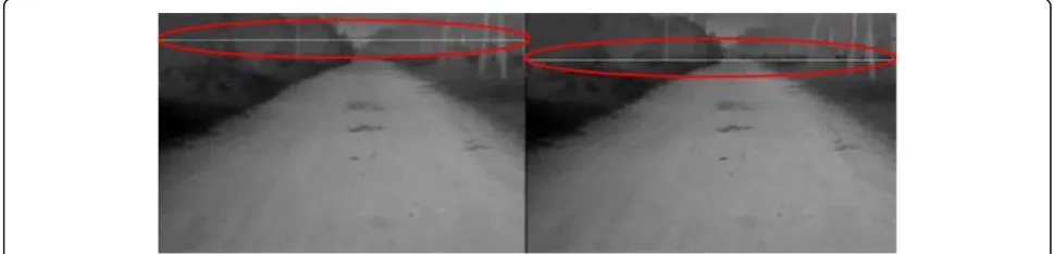
3.2 Comparison of vanishing line detection
For vanishing line detection, Sobel operator is usually used because it has important characteristics, such as fast learning and simple operations that can be used to quickly obtain continuous and smooth boundaries. Sobel operator extracts vertical gradient features, as shown in Fig. 18a. It is easily seen that the vanishing line is very obvious in the vertical gradient. In fact, it appears as the longest straight line located in the upper part of the image. Therefore, the vanishing line can be acquired by
scanning the image to search for the longest straight line as shown in Fig.18b.
The unpaved road suffers from the following issues such as interference caused by shadows and ruts. Sobel operator ignores the complex structural rela-tionships in unpaved roads and therefore can hardly achieve an accurate road detection result. As seen from Fig. 18a, there are some interferences and devia-tions of the vanishing line. In order to solve this problem, we present a normal distribution method as shown in Fig. 19b. By comparing the results in Fig. 19a with those in Fig. 19b, we observe that the normal distribution method that adds a priori infor-mation is more effective than Sobel operator.
3.3 Analysis of image clustering methods
In this work, several methods are considered for detect-ing road regions. To make a comparison, we also report results for some state-of-the-art detection methods, in-cluding those based on (1) DBSCAN method [24] and the result is shown in Fig. 20, (2) K-means method [25] and the result is shown in Fig.21, (3) least squares method [17], and (4) histogram [15]. To achieve a more valid comparison, we adopt the evaluation mechanism proposed in [37] to analyze the results from the above road detection algorithms. Accuracy is defined as follows:
Fig. 20DBSCAN clustering and road boundary recognition.aClustering result.bRoad boundary recognition
Accuracy¼ TPþTN
TPþFPþFNþTN ð16Þ
where true positive (TP) is the number of correctly la-beled road pixels, true negative (TN) is the number of non-road pixels detected, false positive (FP) is the num-ber of non-road pixels classified as road pixels, and false negative (FN) is the number of road pixels erroneously marked as non-road. The better detection algorithm’s performance can obtain the greater accuracy value.
Before calculating the accuracy, we first transform the gray images in Fig.16(the ground truth) into binary im-ages. In our experiment, we regard white (255) and black (0) as the road and the other conditions are the non-road. Here, the road pixels are 1 and the non-road pixels are 0.
Moreover, we record the total time consumption and accuracy of all of the methods, as shown in Table3.
As seen in the aforementioned analysis, it is easy to note that our algorithm achieved obvious improvements and better performance and is more adaptive to real-time road detection.
4 Conclusions
In this paper, we present a method of unpaved road recog-nition and boundary extraction using infrared images. In the proposed approach, the accuracy and robustness of vanishing line detection can be achieved by means of a nor-mal distribution. The improved SVM classifier is trained with the optimal radial kernel parameters and penalty fac-tor parameters for road detection. Meanwhile, the im-proved SVM classifier achieves recognition of the unpredictable road from connected regions. Based on the obtained connected regions, the road probability confi-dence map and trapezoidal forecasting model are formed. Furthermore, we also propose a more suitable FCM cluster to further improve the accuracy of road region recognition. After that, the membership of each connected region can be obtained. The corresponding probability confidence map is able to update the membership degree of the con-nected region. The accuracy of the results is 93.20%. Finally, histogram backprojection method based on the pixel model is used to complement a road region. The experimental re-sults show the advantages and effectiveness of the proposed algorithm.
Abbreviations
DBSCAN:Density-based spatial clustering of applications with noise; FCM: Fuzzy C-means; FN: False negative; FP: False positive; HD: High definition; ML: Machine learning; Rbf: Radial basis function; RGB: Red, green and blue; ROI: Region of interest; SVM: Support vector machine; TN: True negative; TP: True positive
Acknowledgements
The authors would like to thank the editor.
Availability data and materials
Not applicable.
Funding
This study was supported by the National Natural Science Foundation of China (No. 61471110), Foundation of Liaoning Provincial Department of Education (L2014090), and Chinese Universities Scientific Foundation (N160413002, N16261004-2/3/5).
Authors’contributions
In this section, the contributions of each author are exposed. JB is the main author. She obtained the results, made the research and comparison with other authors, and wrote the article. XS helped in optimizing the code with Matlab and fine-tuning the parameters of the algorithms to obtain the best results. YZ and RZ made the bibliography review, analyzed the results, and proposed the optimization of the parameters. They supervised all the work, reviewed the article, and helped in all the process. All authors read and ap-proved the final manuscript.
Ethics approval and consent to participate
Not applicable.
Competing interests
The authors declare that they have no competing interests.
Publisher’s Note
Springer Nature remains neutral with regard to jurisdictional claims in published maps and institutional affiliations.
Author details
1College of Information Science and Engineering, Northeastern University,
Shenyang 110819, China.2Faculty of Robot Science and Engineering,
Northeastern University, Shenyang 110819, China.
Received: 29 August 2017 Accepted: 13 March 2018
References
1. H Kong, JY Audibert, J Ponce, General road detection from a single image. IEEE Trans. Image Process.19(8), 2211–2220 (2010)
2. A Küçükmanisa, G Tarım, O Urhan, Real-time illumination and shadow invariant lane detection on mobile platform. J. Real-Time Image Proc., 1–14 (2017) 3. M Bendjaballah, S Graovac, MA Boulahlib, A classification of on-road
obstacles according to their relative velocities. EURASIP journal on image and video processing2016(1), 41 (2016)
4. C Yan, H Xie, S Liu, et al., Effective Uyghur language text detection in complex background images for traffic prompt identification. IEEE Trans. Intell. Transp. Syst.99, 1–10 (2017)
5. C Yan, H Xie, D Yang, et al., Supervised hash coding with deep neural network for environment perception of intelligent vehicles. IEEE Trans. Intell. Transp. Syst., 1–12 (2017)
6. S Zhou, K Iagnemma,Self-supervised learning method for unstructured road detection using fuzzy support vector machines, RSJ International Conference on Intelligent Robots and Systems(IEEE, IROS, 2010), pp. 1183–1189
7. M Bertozzi, A Broggi, M Cellario, et al., Artificial vision in road vehicles. Proc. IEEE90(7), 1258–1271 (2002)
8. E Shang, X An, J Li, et al., Robust unstructured road detection: the importance of contextual information. Int. J. Adv. Robot. Syst.10(3), 179 (2013) 9. C Yan, Y Zhang, J Xu, et al., A highly parallel framework for HEVC coding
unit partitioning tree decision on many-core processors. IEEE Signal Processing Letters21(5), 573–576 (2014)
Table 3Summary of experimental results on time consumption and assessment
Method Time consumption (ms) Accuracy (%)
DBSCAN-based [24] 29 66.80
K-mean-based [25] 12 88.60
Least squares-based [17] 74 77.20
Histogram-based [15] 37 91.10
10. J Shi, J Wang, F Fu, Fast and robust vanishing point detection for unstructured road following IEEE Transactions on Intelligent Transportation Systems.17(4), 970–979 (2016)
11. X Yang, G Wen,Road extraction from high-resolution remote sensing images using wavelet transform and Hough transform, 2012 5th International Congress on Image and Signal Processing(IEEE, CISP, 2012), Chongqing Univ Posts &
Telecommunications, Chongqing, Peoples Republic of China, pp. 1095–1099 12. Y Wang, C Wen, Vanishing point detection of unstructured road based on
Haar texture. Journal of Image and Graphics18(4), 382–391 (2013) 13. Y Chen, Y Yu, T Li,A vision based traffic accident detection method using
extreme learning machine, International Conference on Advanced Robotics and Mechatronics(IEEE, ICARM, 2016), Macau, China, pp. 567–572
14. K Lu, S Xia, D Chen, et al.,Unstructured road detection from a single image, Control Conference(IEEE, 2016), Kota Kinabalu, Malaysia, pp. 1–6 15. W Zuo, T Yao, Road model prediction based unstructured road detection.
Journal of Zhejiang University SCIENCE C14(11), 822–834 (2013) 16. E Shang, X An, L Ye, et al.,Unstructured road detection based on hybrid
features, Proceedings of the 2012 2nd International Conference on Computer and Information Application(ICCIA, 2012), Taiyuan, Peoples Republic of China, pp. 926–929
17. K Kluge, S Lakshmanan,A deformable-template approach to lane detection, In Proc Intelligent Vehicle '95 Symposium(IEEE,1995), Detroit, MI, USA, pp. 54–59 18. X Hu, R FSA, A Gepperth,A multi-modal system for road detection and
segmentation, Intelligent Vehicles Symposium Proceedings(IEEE, 2014), pp. 1365–1370
19. M Nishida, M Muneyasu,Detection of road boundaries using hyperbolic road model, 2012 International Symposium on Intelligent Signal Processing and Communications Systems(ISPACS, IEEE, 2012), pp. 521–526
20. DY Huang, CH Chen, TY Chen, et al. Vehicle Detection and Inter-vehicle Distance Estimation Using Single-lens Video Camera on Urban/Suburb Roads. J Vis Commun & Image Repres.46, 250–259 (2017)
21. H Zhang, D Hou, Z Zhou, A novel lane detection algorithm based on support vector machine. Piera online1(4), 390–394 (2005)
22. S Zhou, J Gong, G Xiong, et al.,Road detection using support vector machine based on online learning and evaluation, Intelligent Vehicles Symposium(IEEE, IV, 2010), San Diego, CA, pp. 256–261
23. S Yun, Z Guo-Ying, Y Yong,A road detection algorithm by boosting using feature combination, 2007 IEEE Intelligent Vehicles Symposium(IEEE, 2007), Istanbul, Turkey, pp. 364–368
24. S Chakraborty, NK Nagwani, Analysis and study of incremental DBSCAN clustering algorithm. Preprint ArXiv1(2), 1406.4754 (2014)
25. ME Celebi, HA Kingravi, PA Vela, A comparative study of efficient initialization methods for the k-means clustering algorithm. Expert Syst. Appl.40(1), 200–210 (2013)
26. P Conrad, M Foedisch,Performance evaluation of color based road detection using neural nets and support vector machines, Proceedings. 32nd Applied Imagery Pattern Recognition Workshop(IEEE, 2003), Washington, DC, pp. 157–160 27. ZQ Li, HM Ma, ZY Liu,Road lane detection with Gabor filters, International
Conference on Information System and Artificial Intelligence(IEEE, 2017), Hong Kong, Peoples Republic of China, pp. 436–440
28. W Wu, G ShuFeng,Research on unstructured road detection algorithm based on the machine vision, 2009 Asia-Pacific Conference on Information Processing
(APCIP, IEEE, 2009) pp.112-115
29. N Otsu, A threshold selection method from gray-level histograms. IEEE transactions on systems, man, and cybernetics9(1), 62–66 (1979) 30. RD Gupta, M Jamil, M Mohsin, Discharge prediction in smooth trapezoidal
free overfall—(positive, zero and negative slopes). J. Irrig. Drain. Eng.119(2), 215–224 (1993)
31. C Yan, Y Zhang, J Xu, et al., Efficient parallel framework for HEVC motion estimation on many-Core processors. IEEE Transactions on Circuits & Systems for Video Technology24(12), 2077–2089 (2014)
32. T Joachims,Making large-scale SVM learning practical. technical report on Komplexitätsreduktion in Multivariaten Datenstrukturen(SFB, Universität Dortmund, 1998), Cambridge, USA, p. 475
33. U Aich, S Banerjee, Application of teaching learning based optimization procedure for the development of SVM learned EDM process and its pseudo Pareto optimization. Appl. Soft Comput.39, 64–83 (2016) 34. X Liu, KK Shang, J Liu, et al.,Unstructured road detection based on fuzzy
clustering arithmetic, 2014 11th International Conference on Fuzzy Systems and Knowledge Discovery(IEEE, FSKD, 2014), Xiamen, Peoples Republic of China, pp. 114–118
35. YH Lai, PW Huang, PL Lin,An integrity-based fuzzy c-means method resolving cluster size sensitivity problem, 2010 International Conference on Machine Learning and Cybernetics(IEEE, ICMLC, 2010), Qingdao, Peoples Republic of China, pp. 2712–2717
36. J Ji, KL Wang, A robust nonlocal fuzzy clustering algorithm with between-cluster separation measure for SAR image segmentation. IEEE Journal of Selected Topics in Applied Earth Observations and Remote Sensing7(12), 4929–4936 (2014)