ORIGINAL PAPER
Severity analysis of powered two wheeler traffic accidents
in Uttarakhand, India
Sachin Kumar1 &Durga Toshniwal2
Received: 19 August 2016 / Accepted: 21 April 2017 / Published online: 1 May 2017 #The Author(s) 2017. This article is an open access publication
Abstract
Objective Powered Two Wheeler (PTW) vehicles are one of the preferred modes of transport used in India. Also, PTWs accidents are comparatively more frequent than other type of accidents on road. The influencing factors of PTW accidents are also differ from factors that affect other accident types. The objective of this study is to analyze newly available PTWs road accident data from Uttarakhand state in India and reveal-ing the factors that affect the severity of these accidents in various districts of Uttarakhand..
MethodologyTo analyze the factors that affect the severity of road accidents in Uttarakhand, initially we have compared three popular classification algorithms i.e. decision tree (CART), Naïve Bayes and Support vector machine on PTW accident data set. The decision tree algorithm’s (CART) clas-sification accuracy was found better than other two tech-niques. Hence we have preferred CART algorithm to extract the factors that affect the severity of PTWVs accidents in whole Uttarakhand state and its 13 districts separately. Experimental ResultsThe analysis of PTWVs accident data using CART for 13 districts of Uttarakhand and the whole state reveals that every districts have different factors associ-ated with PTW accidents severity. There are some districts in Uttarakhand state which have similar PTW accident patterns, whereas few districts are found to have different PTW acci-dent patterns. These results are very useful to understand the
pattern of PTW accidents in Uttarakhand state. These results can certainly be helpful to overcome the PTWs accident rate in Uttarakhand state.
Keywords Powered two wheeler (PTW) vehicle . Road accident . Classification . Data mining . Decision rules . Traffic safety
1 Introduction
Traffic accident can be considered as an incident in which one or more vehicles collide with another vehicle, person, animal or any other fixed object. Traffic accidents do not only involve human life loss but also property damage. World health orga-nization (WHO) mentioned that there are 1.2 million deaths and around 4 million injuries every year around the world due to traffic accidents [1]. An increasing number in vehicle pur-chase is increasing the number of vehicles on road day by day. Hence, the chances for traffic accident are also increasing.
The traffic accident not only affects the life of victims in-volved in accidents but also affects the life of their associated peoples i.e. family members, business associates etc. Every road accident is left with a record in police database or hospital database. This record consists of various important informa-tion about road accidents i.e. time, date and locainforma-tion of acci-dent, weather information, road characteristics and traffic in-formation at the time of accident. The proper analysis of this information can certainly produce some good results. These results can be utilized to know the factors behind road acci-dents and certain accident preventive efforts can be taken.
Traffic accident analysis is a well known research area. There is a rich literature available that reveals the different techniques and their outcome in road accident analysis. Abdalla et al. [2] analyzed road accident data from Scotland
* Sachin Kumar
1
Centre for Transportation Systems (CTRANS), Indian Institute of Technology Roorkee, Roorkee, Uttarakhand 247667, India
2 Computer Science & Engineering Department, Indian Institute of
and establish the relationship between traffic accident location and its distance from residential areas. Their finding reveals that traffic accidents are more frequent near residential areas in comparison to areas that are not in close proximity of residen-tial areas. Mussone et al. [3] analyzed road accidents that occurred at intersections in Milan, Italy region. They used neural network model to analyze the accident data. Their re-sults showed that the pedestrian hit accident at night time and at non-signalized intersection has the highest frequency of accidents in that region. Several other studies focused on traf-fic accident severity analysis using traditional statistical tech-niques and provide good results [4–12]. However, [13,14] shown that traditional statistical techniques has certain limita-tions in analyzing road accident data. Further, several studies using data mining techniques in road accident analysis has shown that data mining provides productive results than tra-ditional statistical techniques. Data mining techniques [15] are further used to categorize the road accident locations and indentifying factors that affects accidents in those locations [16]. Some authors raised the issue that road accident data is of heterogeneous nature and suggested that clustering prior to analysis of data can certainly remove the heterogeneity [17–19]. Some studies also used data mining techniques to analyze crash counts using time series analysis [20,21].
Powered two wheelers (PTW) are one of the most involved vehicles in road accidents. Although it is direct-ly related to the more number of PTW purchased in comparison to other vehicles. The reason behind the rap-id purchase of PTW is that these vehicles are more easily affordable, small in size, light-weighted, flexible, and speedy than other vehicles in heavy traffic conditions. In other words, a PTW is the vehicle that has been driv-en by people with all economic conditions (rich, middle-class and poor) in both urban and rural roads. Various studies used traditional approaches [22–26] to analyze the crash severity of PTW accidents in developed coun-tries. A study [27] used classification trees to generate rules that predict the crash severity of powered two wheeler accidents.
One of the important things about PTW riders is that, they are more prone to road and traffic accident in com-parison to other vehicles such as cars, SUVs, vans and buses. The motivation behind this study is to identify the different factors that affect severity of road accidents among PTW accidents in Uttarakhand state. We have used decision tree classifier, support vector machine and naïve bayes classifier to predict the factors that affect the sever-ity of PTW road accident in 13 districts of Uttarakhand state. The severity of accidents is categorized into KSI (Killed or severely injured) and SI (Slightly injured). In this study, we have identified several factors that affect the severity of PTW accidents in Uttarakhand, India that will certainly help in overcome the accident rate.
2 Materials and methods
2.1 Data set used
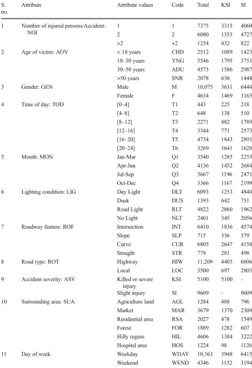
The data set used in this study has been obtained from the GVK-EMRI [28] Dehradun for Uttarakhand state which covers all PTW accidents from January 2010 to December 2014. We are using this 5 year of PTW road accidents data for the severity analysis. This PTW road accident data consists of all 14,709 accident records with 11 attributes from 13 dis-tricts of Uttarakhand. The description of data set and its attri-butes is given in Table1and the distribution of PTW accidents in all 13 districts of Uttarakhand is illustrated in Fig.1.
2.2 Classification techniques
In the domain of data mining [29], classification is a super-vised learning technique that can be defined as follows: given a set of observations, we are interested in extracting certain rules that can be used to predict the class of the each new observation. The set of observations used to extract the rules are known as training set. Another set of observations, known as test set is used to verify the quality and accuracy of the rules. Initially training data and test data both are part of the data set available at the moment. Classification is widely used technique that shows its importance in various fields such as bioinformatics, pattern recognition, image classification etc. In order to achieve the best prediction, more suitable classifi-cation techniques must be selected. The selection of any clas-sification technique depends on the type and nature of data. As our data is more like a categorical data, we are trying to eval-uate the prediction accuracy of three best suitable classifica-tion techniques on our data i.e. decision tree algorithm [30], naïve bayes algorithm [31] and support vector machine algo-rithm [32]. Further, the technique with higher prediction ac-curacy will be used for analysis.
2.3 K-fold cross-validation
validation process is then repeated k times, with each k sub-groups used as a training set exactly once. Further, the k out-comes from the k-fold cross validation can be averaged to produce a single estimation. Usually k remains unfixed in k-fold cross validation, but k = 10 is a standard value that is widely acceptable for k-fold cross validation. This study used k-fold cross validation method to partition data into training and test sets where k = 10 is used.
2.4 Classifier accuracy measures
One of the most important aspects in the classification process is that how well your classifier predicts for unobserved instances. This is known as accuracy of a classifier. Sometimes accuracy itself is not a good measure of classifier goodness. Here, we are providing some classifier accuracy measures that can help in identifying the goodness of a classifier.
Table 1 PTW road accident data
attributes S.
no.
Attribute Attribute values Code Total KSI SI
1 Number of injured persons/Accident: NOI
1 1 7375 3315 4060
2 2 6080 1353 4727
>2 +2 1254 432 822
2 Age of victim: AOV < 18 years CHD 2512 1089 1423
18–30 years YNG 5546 1795 3751
30–50 years ADU 4573 1586 2987
>50 years SNR 2078 630 1448
3 Gender: GEN Male M 10,075 3631 6444
Female F 4634 1469 3165
4 Time of day: TOD [0–4] T1 443 225 218
[4–8] T2 648 138 510
[8–12] T3 2271 482 1789
[12–16] T4 3344 771 2573
[16–20] T5 4734 1843 2891
[20–24] T6 3269 1641 1628
5 Month: MON Jan-Mar Q1 3540 1285 2255
Apr-Jun Q2 4136 1452 2684
Jul-Sep Q3 3667 1196 2471
Oct-Dec Q4 3366 1167 2199
6 Lighting condition: LIG Day Light DLT 6093 1253 4840
Dusk DUS 1393 642 751
Road Light RLT 4822 2860 1962
No Light NLT 2401 345 2056
7 Roadway feature: ROF Intersection INT 6410 1836 4574
Slope SLP 715 336 379
Curve CUR 6805 2647 4158
Straight STR 779 281 498
8 Road type: ROT Highway HIW 11,209 4403 6806
Local LOC 3500 697 2803
9 Accident severity: ASV Killed or severe
injury
KSI 5100 5100
-Slight injury SI 9609 - 9609
10 Surrounding area: SUA Agriculture land AGL 1284 488 796
Market MAR 3679 1370 2309
Residential area RSA 2027 478 1549
Forest FOR 1889 1282 607
Hilly region HIL 4606 1384 3222
Hospital area HOS 1224 98 1126
11 Day of week Weekday WDAY 10,363 3948 6415
2.4.1 Confusion matrix
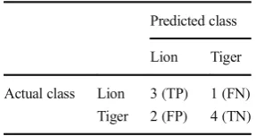
A confusion matrix (or error matrix) [35] is a contingen-cy table that allows visualization of the performance of a classifier. A column in confusion matrix denotes the pre-dicted class instances and a row represents the actual class instances. In order to understand the confusion ma-trix, consider an example of a data sample of 10 animals with 4 lions and 6 tigers. A classification algorithm is trained to distinguish between lions and tigers, a confu-sion matrix will summarize the results of the algorithm for the given sample of data. The confusion matrix for PTW accident data is given in Table 3.
In the above confusion matrix, out of 4 actual lions, clas-sifier predicted 3 lions correctly and predicted 1 lion as a tiger. Out of 6 tigers, 2 were predicted as a lion. All correct predic-tions are located in the diagonal of the Table2. Using this contingency table, other measures can be effectively evaluated.
2.4.2 True positive rate (TPR) and false positive rate (FPR)
TPR measures the fraction of positive that are correctly identified. It is also known as sensitivity of a classifier. It can be calculated using parameters in contingency table using Eq. 1. Whereas, FPR also known as false alarm ratio refers to the probability of falsely rejecting the null
hypothesis. It can be calculated as the number of nega-tive events that are mistakenly categorized as posinega-tive and the total number of actual negative events. The for-mula is given in Eq. 2.
TPR¼ TP
TPþFN ð1Þ
FPR¼ FP
FPþTN ð2Þ
2.4.3 Specificity
The specificity of a classifier is the accuracy of classifier to correctly predict the negative cases in the data set. It can be calculated as
Specificity¼1−FPR¼1 FP
FPþTN ð3Þ
2.4.4 Precision and recall
The precision and recall measures are mostly used metric to measure the performance of a classification algorithm. Precision can be defined as a measure of exactness i.e. if all the predicted labels for a given class X is given, how many instances were correctly classified. Recall which is similar to sensitivity or TPR is the measure of completeness i.e. for all data instances with class value X, how many of these instances are correctly captured.
0 500 1000 1500 2000 2500 3000
Accident
Frequency
KSI SI Fig. 1 PTW accident distribution
in different districts of Uttarakhand
Table 2 Example
confusion matrix Predicted class
Lion Tiger
Actual class Lion 3 (TP) 1 (FN) Tiger 2 (FP) 4 (TN)
The formula for calculating precision is given in equation4 and formula to calculate recall is same as for TPR in Eq.4.
Precision¼ TP
TPþFP ð4Þ
2.4.5 F-measure and MCC
F-measure [35] also known as F-scores is a measure of the classifier test’s accuracy. In order to calculate the F-score of a test, both precision and recall are considered. In other words, F-score can be defined as the harmonic mean of precision and recall. The best value for F-score is close to 1 and worst value is close to 0. F-score can be calculated using Eq.5.
Fscore¼
2TP 2TPþFPþFN
ð Þ ð5Þ
MCC or Matthews correlation coefficient [36] is a measure of the quality of a binary classification, in which variable to be predicted has two values only. In our case, we have two class values for the target attribute i.e. KSI (Killed or severely in-jured) and SI (Slightly inin-jured). It is also considered as a balanced metric to measure the quality of a binary classifica-tion even if the classes are not balanced. Its value ranges between +1 to−1. A value of +1 is considered as a perfect prediction, 0 for average prediction and−1 for no prediction. MCC can be calculated using the values in the confusion matrix using Eq.6.
MCC¼ ffiffiffiffiffiffiffiffiffiffiffiffiffiffiffiffiffiffiffiffiffiffiffiffiffiffiffiffiffiffiffiffiffiffiffiffiffiffiffiffiffiffiffiffiffiffiffiffiffiffiffiffiffiffiffiffiffiffiffiffiffiffiffiffiffiffiffiffiffiffiffiffiffiffiffiffiffiffiffiffiffiffiffiffiffiffiffiðTPTNÞ−ðFPFNÞ
TPþFP
ð ÞðTPþFNÞðTNþFPÞðTNþFNÞ
p ð6Þ
2.4.6 Receiver operating characteristic (ROC) curve
ROC [37] is an important measure to check the accuracy of a classifier. It has been previously used in signal detection the-ory to depict the tradeoff between hit rates and false alarm rates over noisy channel. Now, it is widely used in machine learning field as a useful technique to visualize the perfor-mance of the classifier. ROC curve is a plot between TPR and FPR. To evaluate the performance of the classifier, AUC (area under ROC curve) is calculated. An AUC value close to 1 represent very good performance and a AUC value <0.5 is considered as not good performance.
3 Results and discussion
This section presents the results and experimental analysis of the PTW road accident data mentioned as follows.
3.1 Performance of classification techniques on PTW data
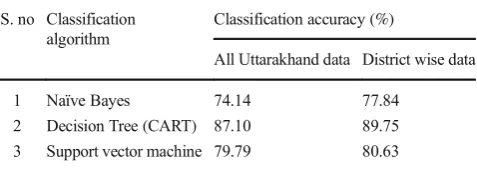
Initially, we applied Classification and Regression Trees (CART) algorithm for decision tree classification, naïve bayes and support vector machine techniques to evaluate the predic-tion accuracy on accidents data. The predicpredic-tion accuracy ob-tained for CART is higher than naïve bayes classifier and support vector machine (Table 3). Hence, we have selected CART decision tree algorithm to analyze our road accident data. The Table3illustrates the prediction accuracy of all three classifiers on PTW accident data set.
3.2 CART performance analysis
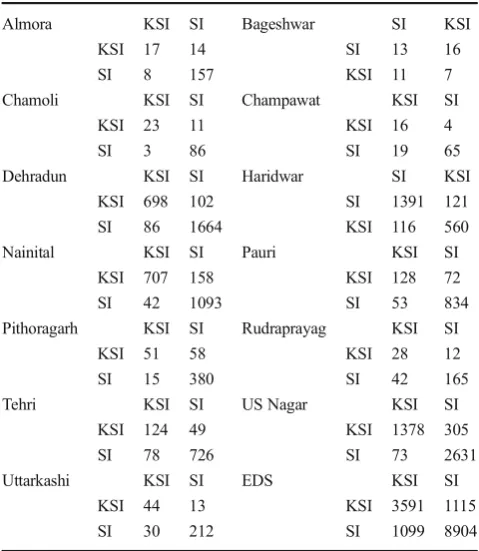
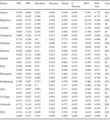
The PTW road ac cident data of 13 districts o f Uttarakhand state is considered for analysis. We build decision tree using CART for all 13 districts and for entire data set (EDS). The confusion matrix obtained after building decision trees for all districts and EDS is shown in Table 4. The different values of classifier ac-curacy measures to illustrate the performance of decision tree classifier on 13 districts of Uttarakhand and EDS have been calculated from confusion matrix and shown in Table 5.
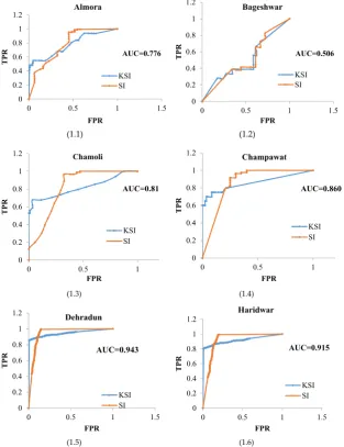
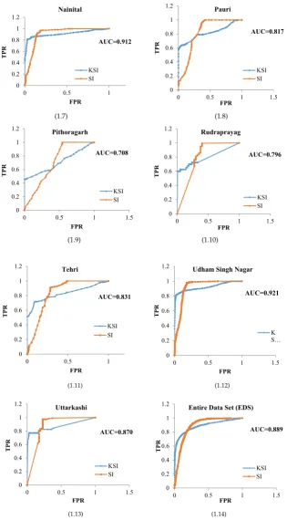
The values of different parameters shown in Table 5 indicate the performance of CART to predict the severity of PTW accidents. The Dehradun, Haridwar, Nainital and Udham Singh Nagar districts which have the high PTW accident rate in Uttarakhand state. The decision tree clas-sifier’s accuracy is found better than other remaining districts. In other districts, the performance of the classi-fier is not so accurate. The one reason can be the small size of the accident records. This certainly reveals the conclusion that if data set is not sufficiently large enough, then the decision tree algorithm may not be ac-curate as desired. The other reason for low accuracy is that the similar values for different attributes are there that predicts the KSI and SI both. The ROC plot is
Table 3 Prediction accuracy of different classifiers
S. no Classification algorithm
Classification accuracy (%)
All Uttarakhand data District wise data
1 Naïve Bayes 74.14 77.84
2 Decision Tree (CART) 87.10 89.75
illustrated to show the performance of decision tree clas-sifier for all 13 districts and EDS in Fig.1.1 to Fig.1.14. The AUC (Area under ROC curve) is shown in each figure. The AUC indicates that the decision tree classifier performs worst for Bageshwar district and best for Dehradun, Nainital, Hardiwar and Udham singh nagar district.
3.3 Decision rules extraction and description
Further, decision rules are extracted from decision tree build for all districts and EDS. The relevant and interest-ing rules have been chosen to describe the patterns of each district and EDS. The description of decision rules are given as follows:
The decision rules for Almora, Bageshwar and Chamoli districts indicate that NOI, TOD, SUA and LIG are the main contributing accidents attributes that is involved in several PTW accidents. The decision rules revealed that PTW acci-dents that occurred during night time with no light conditions were KSI accidents. The locations where road light facilities were present during night time have SI accidents only. In other conditions, it is difficult to conclude between KSI and SI ac-cidents, because similar attribute values were present for both KSI and SI accidents. The other attributes that were not avail-able with the data such as speed and weather information may be the responsible factors for PTW accidents in these districts of Uttarakhand.
The severity of PTW accidents in Champawat and Hardiwar districts were mainly affected by NOI, TOD, ROF and LIG attributes. The decision rules for Champawat district reveals that intersection were mainly involved in KSI acci-dents in during TOD values T1and T6 whereas for other TOD values the accidents were SI. The decision rules for Haridwar district indicate that Intersections in no light condi-tion was more prone to KSI accidents. Other road features such as curve and slope was found to have similar effect on PTW accidents in all lightning conditions for SI accidents with 2 or more victims involved in accidents. Some PTW accidents were KSI accidents that involved 1 victim injured in day light conditions in slope road feature.
The Dehradun district that has the highest PTW road acci-dents in Uttarakhand state was mainly affected by NOI, TOD, ROF, SUA and LIG road accident attributes. The decision rules certainly reveal some interesting information. According to de-cision rules, most of the KSI accidents have occurred in no light conditions in intersections near markets, residential area and ag-riculture land. Curve on road near forest area was also KSI prone area for PTW accidents with 1 victim involved. Other values of different attributes were usually involved in SI accidents.
The factors that affect the severity for PTW accidents in Nainital districts, in addition to other previously mentioned dis-tricts, has few more accident attribute responsible for accidents i.e. Age of victim and ROT. The rules reveals that curve on road are the main factor that contributes to KSI accidents at night and early morning duration. Also, in evening duration the KSI acci-dents on highway roads were involved with minor victims or victims less than 18 years of age.
For Udham singh nagar district, the factors that affect severity of road accidents were quite similar to those fac-tors in Dehradun districts. The colonies and markets areas were the major location where lots of the accidents have occurred but most of these accidents were SI accidents only. The PTW KSI accidents were mainly occurred at a highway that goes through the agriculture land or the for-est area. The YNG and ADU age group victim were main-ly involved in KSI accidents. Very few KSI accidents were involved SNR and CHD group victims.
Rudraprayag, Tehri and Uttarkashi districts were not main-ly affected by ROT, ROF and other important factors which were found for the previous districts. One common factor revealed by decision rules is the LIG condition. Most of the KSI accidents in these districts have occurred in DUSK light-ning condition. Other lightlight-ning conditions were usually in-volved SI accidents. As the accident records for PTW acci-dents for these districts were comparatively low, some other factors remain hidden. The decision rules for Pauri and Pithoragarh districts revealed that these two districts have sim-ilar patterns for PTW accidents. In both districts, the KSI ac-cidents mainly involved the AGE group CHD and SNR and the LIG condition as DUS. Also, these accidents were mainly
Table 4 Confusion matrix for 13 districts and EDS of Uttarakhand
Almora KSI SI Bageshwar SI KSI
KSI 17 14 SI 13 16
SI 8 157 KSI 11 7
Chamoli KSI SI Champawat KSI SI
KSI 23 11 KSI 16 4
SI 3 86 SI 19 65
Dehradun KSI SI Haridwar SI KSI
KSI 698 102 SI 1391 121
SI 86 1664 KSI 116 560
Nainital KSI SI Pauri KSI SI
KSI 707 158 KSI 128 72
SI 42 1093 SI 53 834
Pithoragarh KSI SI Rudraprayag KSI SI
KSI 51 58 KSI 28 12
SI 15 380 SI 42 165
Tehri KSI SI US Nagar KSI SI
KSI 124 49 KSI 1378 305
SI 78 726 SI 73 2631
Uttarkashi KSI SI EDS KSI SI
KSI 44 13 KSI 3591 1115
happened in Q1 and Q4 months of the years. The SI accidents were mainly involved the AGE group ADU, whereas YNG age group was equally involved in both SI and KSI accidents. Further, the rules for the EDS have been analyzed. It was found that for EDS almost all attributes except the MON (month) attribute were involved in KSI and SI accidents for PTW. Most of the KSI accidents were involved NOI values of 1 but very few KSI accidents involved NOI = +2 for EDS. For AGE attribute, the values YNG and ADU were mainly involved in KSI accidents, whereas the number of CHD victims was com-paratively low. SNR victims were found to be involved in both KSI and SI accidents but these accidents are comparatively lower than accidents with other victims. The major road location where most of the KSI accidents have occurred was intersections on highways. Most of the intersections where KSI accidents have occurred were a part of highways. Also the curve on highways was found to be dangerous as it involves most of the KSI acci-dents than SI acciacci-dents. The SUA attribute values MAR and HIL are the locations where most of the accidents have occurred but
the number of SI accidents was more in comparison to KSI accidents in these locations. The SUA values FOR and AGL was found to be dangerous for PTW accidents on local roads. For attribute LIG, around 10% of accidents have occurred in DUS condition in which 46% accidents were KSI, hence the DUS condition could be dangerous for PTW accidents. Although, lots of accidents have occurred in DLT condition but most of the accidents were SI accidents. In RLT condition, it is found that most of the PTW accidents were KSI accidents. Some of the PTW accidents have also occurred in NLT conditions but most of the accidents were SI accidents.
Therefore, it is found that a separate analysis of every district data and a complete analysis of entire data certainly reveal dif-ferent but important information that can be utilized to under-stand the factors that involved in PTW road accidents. The dif-ferent accident attributes have difdif-ferent impact on PTW accidents in every district. It can be concluded that the analysis of entire data can give you a broad overview of the information about the factors involved in road accidents of PTW accidents, whereas a
Table 5 CART performance
metrics for 13 districts and EDS District TPR FPR Specificity Precision Recall F-Measure
MCC ROC
Area
Class
Almora 0.548 0.048 0.952 0.680 0.548 0.607 0.547 0.776 KSI
0.952 0.452 0.548 0.918 0.952 0.935 0.547 0.776 SI
Bageshwar 0.389 0.552 0.448 0.304 0.389 0.341 −0.158 0.506 KSI
0.448 0.611 0.389 0.542 0.448 0.491 −0.158 0.506 SI
Chamoli 0.676 0.034 0.966 0.855 0.676 0.767 0.704 0.819 KSI
0.966 0.324 0.676 0.887 0.966 0.925 0.704 0.819 SI
Champawat 0.800 0.226 0.774 0.457 0.800 0.582 0.479 0.860 KSI
0.774 0.200 0.8 0.942 0.774 0.850 0.479 0.860 SI
Dehradun 0.873 0.049 0.951 0.890 0.873 0.881 0.828 0.943 KSI
0.951 0.128 0.873 0.942 0.951 0.947 0.828 0.943 SI
Haridwar 0.828 0.080 0.92 0.822 0.828 0.825 0.747 0.915 KSI
0.920 0.172 0.828 0.923 0.920 0.921 0.747 0.915 SI
Nainital 0.817 0.037 0.963 0.944 0.817 0.876 0.799 0.912 KSI
0.963 0.183 0.817 0.874 0.963 0.916 0.799 0.912 SI
Pauri 0.640 0.060 0.94 0.707 0.640 0.672 0.604 0.817 KSI
0.940 0.360 0.64 0.921 0.940 0.930 0.604 0.817 SI
Pithoragarh 0.468 0.038 0.962 0.773 0.468 0.583 0.525 0.708 KSI
0.962 0.532 0.468 0.868 0.962 0.912 0.525 0.708 SI
Rudraprayag 0.700 0.203 0.797 0.400 0.700 0.509 0.406 0.796 KSI
0.797 0.300 0.7 0.932 0.797 0.859 0.406 0.796 SI
Tehri 0.717 0.097 0.903 0.614 0.717 0.661 0.584 0.831 KSI
0.903 0.283 0.717 0.937 0.903 0.920 0.584 0.831 SI
US Nagar 0.819 0.027 0.973 0.950 0.819 0.879 0.818 0.921 KSI
0.973 0.181 0.819 0.896 0.973 0.933 0.818 0.921 SI
Uttarkashi 0.772 0.124 0.876 0.595 0.772 0.672 0.590 0.870 KSI
0.876 0.228 0.772 0.942 0.876 0.908 0.590 0.870 SI
EDS 0.763 0.110 0.890 0.766 0.763 0.764 0.654 0.889 KSI
separate analysis of each district can reveal factors associated with PTW accidents in those district only. Therefore, both type of analysis should be performed with EDS and each districts to get a broad and insight information about accident factors.
4 Conclusion
The study used decision tree classification technique to analyze the 5 years PTW road accident data from 13 districts of Uttarakhand state in India. The reason behind selection of deci-sion tree algorithm is that its prediction accuracy is found better than naïve bayes and support vector machine on our data. A total of 14,709 PTW accident record with 11 different attributes were selected to analyze the accident data. A decision tree is a popular data mining technique that is widely used for analysis of road accident data. In this study, we have used decision tree
classification technique for the severity analysis of PTW accident in each district of Uttarakhand. The accident severity in our data is classified into KSI (killed or severely injured) and SI (Slightly injured) class values. The distribution of PTW road accidents in our data was different among all districts. Dehradun, Nainital, Haridwar and Udham singh nagar districts was the district with high number of PTWaccidents, whereas remaining other districts involved comparatively less number of PTW accidents. The se-verity analysis of PTW data revealed different factors contribut-ing to the severity of accidents in different districts. The decision tree classifier’s performance in those districts with good number of accident records was very good (illustrated in Fig.2) whereas for the districts with very less number of accident records was not so good. Some districts such as Uttarakashi, Tehri, Rudraprayag, Almora, Bageshwar and Chamoli contains very few accident records, therefore neither the classifier’s accuracy was good nor the decision rules generated revealed very fruitful information
(1.1) (1.2)
(1.3) (1.4)
(1.5) (1.6)
0 0.2 0.4 0.6 0.8 1 1.2
0 0.5 1 1.5
TPR
FPR Almora
KSI SI
0 0.2 0.4 0.6 0.8 1 1.2
0 0.5 1 1.5
TPR
FPR Bageshwar
KSI SI
0 0.2 0.4 0.6 0.8 1 1.2
0 0.5 1
TPR
FPR Chamoli
KSI SI
AUC=0.81
0 0.2 0.4 0.6 0.8 1 1.2
0 0.5 1
TPR
FPR Champawat
KSI SI
AUC=0.860
0 0.2 0.4 0.6 0.8 1 1.2
0 0.5 1 1.5
TPR
FPR Dehradun
KSI
SI 0
0.2 0.4 0.6 0.8 1 1.2
0 0.5 1 1.5
TPR
FPR Haridwar
KSI SI
AUC=0.915
AUC=0.776 AUC=0.506
AUC=0.943
about the PTW accidents in these districts. Hence, it is certain that more information is required to get more fruitful results. The decision rules revealed that different attributes were found to be involved in KSI accidents for different districts, but the analysis of EDS showed that all accident attributes except MON (month)
was involved in KSI accidents in Uttarakhand state. It simply means, that PTW accidents have no impact of month on accident severity or it is not very contributing factor for KSI accidents. These rules provide some useful information which can be used to understand the different circumstances that contributes to
(1.7) (1.8)
(1.9) (1.10)
(1.11) (1.12)
0 0.2 0.4 0.6 0.8 1 1.2
0 0.5 1
TPR
FPR
Nainital
KSI SI
AUC=0.912
0 0.2 0.4 0.6 0.8 1 1.2
0 0.5 1 1.5
TPR
FPR
Pauri
KSI SI AUC=0.817
0 0.2 0.4 0.6 0.8 1 1.2
0 0.5 1 1.5
TP
R
FPR
Pithoragarh
KSI SI AUC=0.708
0 0.2 0.4 0.6 0.8 1 1.2
0 0.5 1 1.5
TPR
FPR
Rudraprayag
KSI SI AUC=0.796
0 0.2 0.4 0.6 0.8 1 1.2
0 0.5 1
TP
R
FPR
Tehri
KSI SI AUC=0.831
0 0.2 0.4 0.6 0.8 1 1.2
0 0.5 1 1.5
TP
R
FPR
Udham Singh Nagar
K
S… AUC=0.921
(1.13) (1.14)
0 0.2 0.4 0.6 0.8 1 1.2
0 0.5 1 1.5
TP
R
FPR
Uttarkashi
KSI SI AUC=0.870
0 0.2 0.4 0.6 0.8 1 1.2
0 0.5 1 1.5
TP
R
FPR
Entire Data Set (EDS)
KSI SI AUC=0.889
PTW accident to occur. Further, this information can be utilized to develop some policies to prevent and overcome the PTW accidents in Uttarakhand state and its districts. The study present-ed a classification baspresent-ed approach on PTW accident data from Indian state. The quality of experiments and results in this study are subject to the quality and attributes of the data in India. However, European countries (Mostly western) have well main-tained road accident data sources with quality information. The methodology adopted in this study could be utilized to analyzed quality PTW data from European countries to provide more quality results that would certainly useful to reveal different im-portant factors for PTW accidents.
Acknowledgments We thankfully acknowledge the GVK-EMRI, Dehradun to provide the data for our research work.
Compliance with ethical standards
Conflicts of Interest Authors do not have any conflict of interest in publication of this manuscript.
Open AccessThis article is distributed under the terms of the Creative C o m m o n s A t t r i b u t i o n 4 . 0 I n t e r n a t i o n a l L i c e n s e ( h t t p : / / creativecommons.org/licenses/by/4.0/), which permits unrestricted use, distribution, and reproduction in any medium, provided you give appro-priate credit to the original author(s) and the source, provide a link to the Creative Commons license, and indicate if changes were made.
References
1. World Health Organization. Global Status Report on Road Safety 2015. Available online: http://www.who.int/violence_injury_ prevention/road_safety_status/2015/GSRRS2015_Summary_EN_ final2.pdf?ua=1(accessed on 01.07.2016)
2. Abdalla IM, Raeside R, Barker D, McGuigan DR (1997) An inves-tigation into the relationships between area social characteristics and road accident casualties. Accid Anal Prev 29:583–593 3. Mussone L, Ferrari A, Oneta M (1991) An analysis of urban collisions
using an artificial intelligence model. Accid Anal Prev 31:705–718 4. Poch M and Mannering F (1996) Negative binomial analysis of
intersection-accident frequencies. J Transp Eng 122
5. Karlaftis M, Tarko A (1998) Heterogeneity considerations in acci-dent modeling. Accid Anal Prev 30:425–433
6. J. Ma, K. Kockelman (2006) Crash frequency and severity model-ing usmodel-ing clustered data from Washmodel-ington state. In: IEEE Intelligent Transportation Systems Conference. Toronto Canadá
7. Abdel-Aty MA and Radwan AE (2000) Modeling traffic accident occurrence and involvement. Accid Anal Prev 32
8. Miaou SP (1994) The relationship between truck accidents and geometric design of road sections–poisson versus negative binomi-al regressions. Accid Anbinomi-al Prev 26
9. Chen W, Jovanis P (2002) Method of identifying factors contribut-ing to driver-injury severity in traffic crashes. Transp Res Rec. 1717 10. Maher MJ and Summersgill IA (1996) Comprehensive methodology
for the fitting of predictive accident models. Accid Anal Prev 28 11. Joshua SC and Garber NJ (1990) Estimating truck accident rate and
involvements using linear and poisson regression models. Transp Plan Technol 15
12. Jones B, Janssen L and Mannering F (1991) Analysis of the frequency and duration of freeway accidents in Seattle. Accid Anal Prev 23 13. Miaou SP and Lum H (1993) Modeling vehicle accidents and
high-way geometric design relationships, Accid Anal Prev 25 14. Chang LY and Chen WC (2005) Data mining of tree based models
to analyze freeway accident frequency. J Saf Res 25
15. Kumar S and Toshniwal D (2015) Analyzing road accident data using association rule mining, international conference on comput-ing communication and security (ICCCS-2015), Dec-2015, Mauritius
16. Kumar S, Toshniwal D (2016) A data mining approach to characterize road accident locations. Journal of Modern Transportation 24:62–72 17. Oña JD, López G, Mujalli R and Calvo FJ (2013) Analysis of traffic
accidents on rural highways using latent class clustering and Bayesian networks. Accid Anal Prev 51
18. Kumar S, Toshniwal D (2015) A data mining framework to analyze road accident data. Journal of Big Data 2:1–18
19. Kumar S, Toshniwal D, Parida M (2016) A comparative analysis of heterogeneity in road accident data using data mining techniques. Springer, Evol Syst doi:10.1007/s12530-016-9165-5
20. Kumar S, Toshniwal D (2016) A novel framework to analyze road accident time series data. Journal of Big Data 3:1–11
21. Kumar S, Toshniwal D (2016) Analysis of road accident counts using hierarchical clustering and cophenetic correlation coefficient (CPCC). Journal of Big Data 3:1–11
22. Quddus MA, Noland RB, Chin HC (2002) An analysis of motor-cycle injury and vehicle damage severity using ordered probit models. J Saf Res 33:445–462
23. Rifaat SM, Tay R, de Barros A (2012) Severity of motorcycle crashes in Calgary. Accid Anal Prev 49:44–49
24. Savolainen P, Mannering F (2007) Probabilistic models of motor-cyclists’injury severities in single- and multi-vehicle crash. Accid Anal Prev 39:955–963
25. Yannis G, Golias J, Papadimitriou E (2005) Driver age and vehicle engine size effects on fault and severity in young motorcyclists accidents. Accid Anal Prev 37:327–333
26. de Lapparent M (2006) Empirical Bayesian analysis of accident severity for motorcyclists in large French urban areas. Accid Anal Prev 38:260–268
27. Montella A, Aria M, Ambrosio AD, Mauriello F (2012) Analysis of powered two wheeler crashes in Italy by classification trees and rules discovery. Accid Anal Prev 49:58–72
28. http://www.emri.in/accessed on 14.07.2016.
29. Han J, Kamber M (2001) Data mining: concepts and techniques. Morgan Kaufmann Publishers, USA
30. Quinlan JR (1986) Induction of decision trees. Mach Learn 1(1): 81–106 doi:10.1023/A:1022643204877
31. Russell S and Norvig P (1995) Artificial intelligence: a modern approach, (2nd ed.). Prentice Hall
32. Cortes C, Vapnik V (1995) Support-vector networks. Mach Learn 20:273–297
33. Tan PN, Steinbach M and Kumar V (2006) Introduction to data mining. Pearson Addison-Wesley
34. R. Kohavi, A study of cross-validation and bootstrap for accuracy estimation and model selection. Proceedings of the Fourteenth International Joint Conference on Artificial Intelligence (San Mateo, CA: Morgan Kaufmann) 2 (12): 1137–1143, 1995. 35. Powers MW (2011) Evaluation: from precision, recall and
F-measure to ROC, Informedness, markedness & correlation. J Mach Learn Technol 2:37–63
36. Matthews BW (1975) Comparison of the predicted and observed secondary structure of T4 phage lysozyme. Biochimica et Biophysica Acta (BBA) - Protein Structure 405:442–451 37. Fawcett T (2006) An introduction to ROC analysis. Pattern Recogn