https://doi.org/10.1186/s13408-018-0058-8
R E S E A R C H Open Access
Kernel Reconstruction for Delayed Neural
Field Equations
Jehan Alswaihli1,2 ·Roland Potthast1,3·
Ingo Bojak4·Douglas Saddy4·Axel Hutt1,3
Received: 26 June 2017 / Accepted: 17 January 2018 /
© The Author(s) 2018. This article is distributed under the terms of the Creative Commons Attribution 4.0 International License (http://creativecommons.org/licenses/by/4.0/), which permits unrestricted use, distribution, and reproduction in any medium, provided you give appropriate credit to the original author(s) and the source, provide a link to the Creative Commons license, and indicate if changes were made.
Abstract Understanding the neural field activity for realistic living systems is a
chal-lenging task in contemporary neuroscience. Neural fields have been studied and de-veloped theoretically and numerically with considerable success over the past four decades. However, to make effective use of such models, we need to identify their
constituents in practical systems. This includes the determination of model
param-eters and in particular the reconstruction of the underlying effective connectivity in biological tissues.
In this work, we provide an integral equation approach to the reconstruction of the
neural connectivity in the case where the neural activity is governed by a delay
neu-ral field equation. As preparation, we study the solution of the direct problem based on the Banach fixed-point theorem. Then we reformulate the inverse problem into a
family of integral equations of the first kind. This equation will be vector valued when
several neural activity trajectories are taken as input for the inverse problem. We
em-B
J. AlswaihliR. Potthast
I. Bojak
D. Saddy
A. Hutt
1 Department of Mathematics and Statistics, University of Reading, Reading, UK 2 Department of Mathematics, Faculty of Education, Misurata University, Misurata, Libya 3 Division for Data Assimilation (FE12), Deutscher Wetterdienst, Offenbach, Germany 4 Centre for Integrative Neuroscience and Neurodynamics (CINN), Department of Psychology,
ploy spectral regularization techniques for its stable solution. A sensitivity analysis of the regularized kernel reconstruction with respect to the input signaluis carried out, investigating the Fréchet differentiability of the kernel with respect to the signal. Finally, we use numerical examples to show the feasibility of the approach for ker-nel reconstruction, including numerical sensitivity tests, which show that the integral
equation approach is a very stable and promising approach for practical
computa-tional neuroscience.
Keywords Neural fields·Integral equations·Fixed-point theorem·Inverse problems·Regularization
1 Introduction
In recent years, studying the activity of neural tissue and development of mathemat-ical and numermathemat-ical techniques to understand neural processes has led to improved neural field models. Since the early work of Wilson, Cowan and Amari in the 1970s neural field models have become an effective tool in neuroscience [1–4].
The neural networks occurring in nature are typically complex systems sporting a large variety of properties in space and time. Simplifying their analysis is generally difficult—in particular when one considers the many billions of neurons of the entire human nervous system, where each of these neurons can be considered as a complex biological system by and in itself, cf. [5]. However, neural field models describe these complicated system mathematically in a few equations, essentially by using the large number of neurons to achieve simplification in terms of mass action. Thus these models consider averages of the neural activity as a dynamical variable, and averages of neural properties as parameters. The derivation of neural models from properties of single neurons and their networks, and the analysis of the resulting activity, remains a major focus of current research [1,6–11].
In this century, there are many papers on the neural field equation with and with-out delays. Some of the studies provide a framework for the existence, uniqueness and stability of the solutions of the neural field equation such as [8–15], while oth-ers consider building effective methods to investigate and assimilate the neural field activities, see for example [16–21] with techniques of Data assimilation and Inverse Problems applied to the case without delays. Recently, Nogaret et al. [7] built a model construction method using an optimization technique to assimilate neural data to de-termine parameters in a detailed neural model including delay.
A challenge often encountered in the study of living systems is to estimate a
given at each location in a given spatial domain and the underlying spatial connec-tivity is derived. The problem of having limited measurements is part of subsequent work combining inverse techniques with state estimation techniques. Here, we focus on the problem to reconstruct the kernelwwhenuis known.
The present work considers neural field models that involve delayed spatial in-teractions and where the delay may depend on the distance between spatial locations [11,14,22]. We will assume that the delay functionD(r, r)between spatial locations r,ris known. For instance, this is the case when the delay is linked to the geometry of the problem, e.g., whenD(r, r)∼ r−r, the distance between the pointsrand rin some domainΩ. This assumption is common in practice, since for direct neural connections the delay is essentially the distance divided by the signal propagation speed, which can be assumed to be a universal constant in a first approximation.
Neural field models consider spatially nonlocal interactions, which may be ex-pressed equivalently either by higher orders of spatial derivatives or by spatial inte-grals [22,23]. In the first part of this paper, we will show how the methods used in [12] can be modified to study existence and stability of solutions in a neural field model with delay. The basic idea is to split the integral operators under considera-tion into parts with positive and negative temporal arguments. As a result we obtain a direct and flexible basic existence proof for a delay neural field equation, which includes a constructive method based on integral equations only. These results have been derived by other authors [8,10,11,24] with more sophisticated techniques, but it is non-trivial that the arguments used for neural fields without delay are applicable to the delay case, and the approach in our Sect.2, based on several relatively simple functional analytic arguments, is of interest by itself.
Second, we will show that the kernel reconstruction problem for the delay neural field equation can be reformulated into a family of integral equations of the first kind. When several trajectories of neural activity are given, the family of integral equations is vector valued. This turns out to be an ill-posed problem, for smooth neural activ-ity it is even exponentially ill posed. To formulate stable numerical methods for its solution, we need to employ regularization. Here, we use a spectral approach to clas-sical Tikhonov regularization [25–27]. We then study the sensitivity of the mapping u→wshowing that its regularized version is Fréchet differentiable, and we calculate the derivative by means of integral equations.
In the third part of the paper, we show by a numerical study that the kernel re-construction from a delay neural field is feasible. We numerically solve the family of integral equations under consideration by a collocation method and provide a study of reconstructions based on the regularization of the ill-posed integral operators un-der consiun-deration. This includes a study of the influence of measurement noise on the reconstruction quality and tests of the role of the regularization parameter.
2 The Mathematical Model
In neural dynamics, neurons send electrical spikes to each other through axons ter-minating in synapses. Letu(rj, t )denotes the average membrane potential of thejth
neuron located at positionrj at timet in a network ofN units. LetW (rj, ri)be the
average connectivity strength between neuron at positionri and neuron at positionrj.
The functionf is the activation rate or firing rate function, which describes the con-version of the membrane potentialu(rj, t )into a spike train S(ri, t )=f[u(ri, t )],
which is then leading to an excitation of neurons at location rj with strength
W (rj, ri)S(ri, t ). The dynamics of the excitation is now described by the ODEs
τdu
dt(rj, t )= −u(rj, t )+
N
i=1
W (rj, ri)f
u(ri, t )
. (1)
This combination of an exponential decay with characteristic timeτ and a sum of excitation terms is commonly called a ‘leaky integrator model’. The sum represents the net-input to unitj, i.e., the weighted sum of activity delivered by all unitsithat are connected to unitjwith a connection strengthW (rj, ri); cf. [12,28]. The continuous
version of (1) is obtained by considering neurons which are continuously distributed over the spaceΩ, e.g., in a plane withΩ∈R2orΩ∈R3and by replacing the sum by an integral. This leads to the simplest form of the Amari neural field equation [4],
τ∂u
∂t(r, t )= −u(r, t )+
Ω
wr, rfur, tdr, r∈Ω. (2)
Hereu(r, t )indicates a neural field representing the activity of the population of neu-rons at positionrand timet. The second term on the right-hand side represents the synaptic input, where f is the activation (or firing rate) function of a single neu-ron. The kernelw(r, r)is often referred to as the synaptic footprint [29–31] or the
connectivity function [12,14,32,33]. It presents the strength of the connection be-tween neurons located atrandr. The functionwincorporates three different kinds of meaning: the existence of a connection in the first place, ifw=0, the functional effect of either excitation, ifw >0, or inhibition, ifw <0, and finally the strength of the connectivity via|w|[4,12,34].
Although the neural field equation (2) represents several biological mechanisms, this form still neglects any delay between spatial locations. In reality, finite transmis-sion speeds in axons, synapses and dendrites cause a functionally significant delay. Taking it into account, the neural field equation involving delayed interactions be-comes
τ∂u
∂t(r, t )= −u(r, t )+
Ω
wr, rfur, t−Dr, rdr, r∈Ω, (3)
conditions. These depend on the geometry of the spatial domain and the specific tem-poral dynamics under study. They are considered in detail in the subsequent sections. The existence of solutions to the neural field equation (3) has been investigated in various papers already [10–12]. For example, Potthast and beim Graben [12] provide the proof of existence and its analysis in the case of no delay, i.e. forD(r, r)=0. In addition, Faugeras and Faye [10], in their Theorem 3.2.1, state the general existence of solutions with a reference to the generic theory of delay equations, based on work such as [35]. We also point out the work of Van Gils et al. [8] employing the sun–star calculus for their analysis and [24] in which the local bifurcation theory for delayed neural fields was developed. Here, we develop arguments on how to use the basic functional analytic calculus to work for the delay case as well, with the goal to present a short and elementary approach which is easily accessible.
3 The Delay Neural Field Equation
In this work, we study the neural field equation (3) on some bounded domainΩ⊂Rm in a space with dimensionm=2 orm=3. We assume that the transmission delay D(r, r)of neural excitation or inhibition betweenrandris bounded onΩ×Ω, i.e. there is a constantcT such that
Dr, r≤cT, r, r∈Ω. (4)
At timet∈R, the neural fieldsu(r, t )at a pointr∈Ωmight receive excitations from the past with a maximal delay ofcT. Working on the time interval[0, ρ]withρ >0,
equation (3) is complemented by initial conditions in the time interval[−cT,0]. The
initial condition for the delay neural field equation is given by
u(r, t )=u0(r, t ), (r, t )∈Ω× [−cT,0]. (5)
We lay ground for our inverse and sensitivity analysis by a basic derivation of the unique solvability of equation (3), using tools from functional analysis and integral equations. Our investigation here makes a smoothness assumption for the activity functionf and the connectivity kernelw. We consider a continuous activation func-tionf (s)fors∈Rand an activation thresholdη. This function may be interpreted as the mass action probability of neurons firing if their membrane potential is over the threshold, and can be derived from a stochastic neuron models [6,36]. Typically [1, 29],f is approximated by the logistic sigmoidal function
f (s)= 1
1+e−σ (s−η), s∈R, (6)
with some steepness parameterσ >0 and thresholdη. For the functionf :R→R+ we note that
f (s)⊂ [0,1], s∈R. (7)
• (H1)w(r,·)∈L1(Ω),∀r∈Ω⊂Rm,
such that we obtain a well-defined integral of the form
g(r, s):=
Ω
wr, rfur, s−Dr, rdr, r∈Ω, s∈R.
The condition
• (H2) supr∈Ωw(r,·)L1(Ω)≤C1,
with some constantC1leads togbeing bounded onΩ×R. We needg(r, s)to be continuous in dependence ofr ands, which for continuous functionsu and D is achieved by the additional condition
• (H3)w(r,·)−w(r∗,·)L1(Ω)→0 for|r−r∗| →0.
Now, existence is given by the following result.
Theorem 3.1 (Existence) If the kernelwsatisfies (H1)–(H3), and if the delay term
Dis bounded continuous, i.e., if we haveD∈BC(Ω×Ω,R+), then for anyT >0
and for any initial fieldu0as given by the initial condition (5) there exists a unique solutionu∈C1(Ω× [0, T])to the delay neural field (3) on[0, T].
Proof We first need some preparations. We will need to split the functionu(r, s− D(r, r))into the part where the time variablet=s−D(r, r)is in(0, T]and where t=s−D(r, r)is in[−cT,0]. This is carried out by defining
χ+(r, t ):= 1, t >0,
0, t≤0, (8)
andχ−(r, t ):=1−χ+(r, t ). The function χ− is equal to 1 for negative time argu-ments and we have 1=χ++χ−. For studying the existence of solutions of the delay neural field equation (3) we define the operators
(A1u)(r, t ):=
t
0
−u(x, s)
τ ds, r∈Ω andt≤0, (9)
and
A±2u(r, t ):= 1 τ
t
0
Ω
wr, rχ±r, s−Dr, r
·fur, s−Dr, rdrds (10)
forr∈Ω andt∈ [0, T]. By integration with respect to time the solution of (3) can be reformulated as
u(r, t )−u(r,0)
=1
τ t
0
−u(r, s)+
Ω
wr, rfur, s−Dr, rdr
forr∈Ω andt∈ [0, ρ]with an auxiliary parameterρ. Differentiating equation (11) with respect to time, we return to the delay neural field equation (3). We can now split the operators as follows:
1 τ t 0 Ω
wr, rfur, s−Dr, rdrds
=A+2u(r, s)+A−2u(r, s)
=A+2u(r, s)+A−2u0
(r, s), (12)
where the last equality is obtained from
τA−2u(r, t )= t
0
Ω
wr, rχ−r, s−Dr, rfur, s−Dr, rdrds
=
Ω t
0
wr, rχ−r, s−Dr, rfur, s−Dr, rds dr
=
Ω
D(r,r)
0
wr, rfur, s−Dr, rds dr
=
Ω
D(r,r)
0
wr, rfu0
r, s−Dr, rds dr
=
Ω t
0
wr, rχ−r, s−Dr, rfu0
r, s−Dr, rds dr
=
t
0
Ω
wr, rχ−r, s−Dr, rfu0
r, s−Dr, rdrds
=τA−2u0
(r, t )
usingu(r, t )=u0(r, t )fort≤0. WithA:=A1+A+2 the delay neural field equation
is equivalent to the fixed-point equation
u(r, t )=u(r,0)+A−2u0
(r, t )+(Au)(r, t ), r∈Ωandt∈ [0, ρ]. (13)
Here, the function u(r, t ) needs to be considered on Ω× [0, ρ]only and we can study the fixed-point equation in BC(Ω× [0, ρ]). Any solution to equation (13) will be continuously differentiable with respect to time and satisfy the delay neural field equation (3). We now show that for sufficiently small parameterρ >0 the operator Ais a contraction on the space BC(Ω× [0, ρ])equipped with its canonical norm
vρ:= sup r∈Ω,t∈[0,ρ]
v(r, t ). (14)
We will carry out these arguments in four steps, I–IV.
I. For the linear operatorA1 given by equation (9), we follow [12], Lemma 2.5,
and estimate
(A1u)ρ= sup
r∈Ω,t∈[0,ρ]
(A1u)(r, t )≤
ρ
τ r∈Ω,tsup∈[0,ρ]
u(r, t )=ρ
i.e., the operatorA1 maps the space BC(Ω× [0, ρ])boundedly into itself and by
equation (15) the operator norm is bounded byρ/τ.
II. We define
J u(r, t ):=1 τ
Ω
wr, rχ+r, t−Dr, rfur, t−Dr, rdr, (16)
forx∈Ωandt≥0, and follow [12], Lemma 2.5, to estimate J u1(r, t )−J u2(r, t )
≤ 1
τ
Ω
wr, rχ+r, t−Dr, r
·fu1
r, t−Dr, r−fu2
r, t−Dr, rdr (17)
forx∈Ωandt∈ [0, ρ]. First, using the Lipschitz continuity of the functionf with Lipschitz constantL >0, usingC1given in (H2) we obtain
J u1(r, t )−J u2(r, t )
≤L
τ
Ω
wr, rχ+r, t−Dr, r
·u1
r, t−Dr, r−u2
r, t−Dr, rdr
≤LC1
τ rsup∈Ω
χ+r, t−Dr, ru1
r, t−Dr, r−u2
r, t−Dr, r
≤LC1
τ u1−u2Ω×[0,ρ] (18)
forr∈Ωandt∈ [0, ρ].
III. Integration of equation (18) with respect tot∈ [0, ρ]leads to
A+2(u1)−A+2(u2)ρ≤
ρLC1
τ u1−u2ρ, (19)
where · ρas defined in equation (14). Now, for the operatorAwe obtain the
esti-mate
A(u1)−A(u2)ρ=A1(u1−u2)+A+2(u1)−A+2(u2)ρ
≤ρ
τu1−u2ρ+ ρLC1
τ u1−u2ρ
≤qu1−u2ρ, (20)
with
q:=ρ
In the case whereρ is small enough to guarantee that q <1 by equation (20), we have shown thatAis a contraction on BC(Ω× [0, ρ], · ρ).
IV. According to the Banach fixed-point theorem, there is one and only one fixed pointu∗for the fixed-point equation (13). We have shown the existence of a unique solution u(x, t ) for allt ∈ [0, ρ]. Now, the same argument applied to the interval
[ρ,2ρ] and subsequent intervals[2ρ,3ρ] etc. in the same way. This leads to the
existence and uniqueness result on the interval[0, T].
Remark We note that the proof also works when some bounded continuous forcing
termI (r, t ),r∈Ω,t∈ [0, T], is added to the neural field equation (3). It leads to an additional term in Eq. (13), for which all arguments remain valid.
It is well known [21, 27] that Banach’s theorem also provides a constructive method to calculate the fixed point by successive iterations. Letu1be a starting
func-tion. Then the sequence defined by
un+1:=u0+A−2(u0)+A(un), n=1,2,3, . . . , (22)
converges to the unique fixed pointu∗. An error estimate for this iteration process based on equation (20) is obtained from
un+1−u∗=u0+A−2(u0)+A(un)−
u0+A−2(u0)+A
u∗
=A(un)−A
u∗
≤qun−u∗. (23)
Induction immediately leads to the full error estimate
un+1−u∗≤qnu1−u∗, n∈N. (24)
For our numerical calculations we have, however, instead used Runge–Kutta or Euler methods applied to the differential form of the delay neural field equation.
4 The Inverse Problem of Kernel Reconstruction with Delays
We now come to the kernel reconstruction from given dynamical neural patterns with delay. We first formulate a regularized kernel reconstruction approach based on
integral equations in Sect.4.1, then we carry out a sensitivity analysis in Sect.4.2.
4.1 Kernel Reconstruction with Delays
• the nonlinear activation functionf :R→R+is known, and
• the delay functionD:Ω×Ω→ [0, cT]is given.
The task is to find a kernelw(r, r)for (r, r)∈Ω given the time-dependent neural activation patternsu(ξ )(r, t )for(r, t )∈Ω×[0, T]corresponding to initial conditions u(ξ )0 (r, t )for(r, t )∈Ω× [−cT,0]according to equation (5), whereξ =1, . . . , N.
Here, we reformulate the inverse problem into a family of integral equations of the
first kind and study their solution by regularization methods. As a first step, we define
φ(ξ )(r, s):=fu(ξ )(r, s), (r, s)∈Ω× [−cT, T], (25)
and
ψ(ξ )(r, t ):=τ∂u
(ξ )
∂t (r, t )+u
(ξ )(r, t ), (r, t )∈Ω× [0, T], (26)
forξ=1,2, . . . , N. With the integral operatorWdefined by
(W φ)(r, t ):=
Ω
wr, rφr, t−Dr, rdr, (r, t )∈Ω× [0, T], (27)
the inverse problem is reformulated as the equation
ψ(ξ )(r, t )=W φ(ξ )(r, t ), (r, t )∈Ω× [0, T], (28)
withξ=1,2, . . . , N, where the kernelw(r, r)withr, r∈Ω of the linear operator Wis unknown. Equation (28) can be written as
ψ=W φ, (29)
withφ=(φ(1), φ(2), . . . , φ(N ))T andψ=(ψ(1), ψ(2), . . . , ψ(N ))T, where we search for the unknown operatorW. An alternative is to rewrite equation (28) as
ψr(t )=
Ω
φr, t−Dr, rwr
rdr, t∈ [0, T], (30)
for every fixedr∈Ω with
ψr(t ):=ψ (r, t ), t∈ [0, T], (31)
and
wr:=w
r, r, r, r∈Ω. (32)
Equation (30) is a family of integral equations for the unknown kernelw(r, r), where each functionwr=w(r,·)provides a different integral equation with a different
inte-gral kernel and a different left-hand side. Its structure is given by the inteinte-gral operator
(Vrg)(t ):=
Ω
Kr
with kernel
Kr
t, r:=φr, t−Dr, r, t, r∈ [0, T] ×Ω, (34)
forr∈Ω. ForN >1 this kernel is a vector of functionsφ(ξ )(r, t−D(r, r))with ξ=1, . . . , N. Now, our inverse problem equation (30) is given by
ψr =Vrwr (35)
forr∈Ω. For eachr∈Ω equation (35) is a Fredholm integral equation of the first kind with continuous kernelφ. The operatorVr is a compact operator on the spaces
C(Ω),L1(Ω)orL2(Ω)into BC([0, T]). It is well known (cf. [21,25,27,37]) that this equation is ill posed, i.e. it does not need to have unique solutions and if it has a solution in general this solution does not depend continuously on the right-hand side. Ill-posed equations need some regularization method (cf. [26]) in order to obtain a stable solution. A standard approach to regularization is built on the singular sys-tem (cf. [27]) of the operator under consideration. In summary, for a compact linear operatorA:X→Y between Hilbert spacesXandY, and its adjointA∗, the singu-lar valuesμn of the operatorAare the non-negative square roots of the eigenvalues
of the self-adjoint compact operator A∗A:X→X. This leads to a representation of the operator as a multiplication of two orthonormal systemsgn:n∈NinXand
yn:n∈NinY. Hence, this corresponds to a spectral representation of the operator
Ain the form
Ag=
∞
n=1
μng, gnyn, (36)
forg∈X. For the orthonormal systemsgnandynwe obtain
Agn=μnyn, A∗yn=μngn. (37)
Here, in the caseAthat is injective, the inverse ofAis given by
A−1y=
∞
n=1
1 μn
y, yngn (38)
or, ifAis not injective, the inverseA−1in equation (38) projects onto the orthogonal space N (A)⊥= {g|g, g∗ =0,∀g∗∈N (A)}. Because of the compactness of the operatorsA, the singular values are a sequence mostly accumulating at zero. So, the behaviour of|μ1
n| → ∞,n→ ∞enlarges small errors causing the instability of
applying the inverse. The practical behaviour of the sequence of singular valuesμn
provides important insight into the nature of the instability. For the application at hand the problem is strongly ill posed for strong smoothness of the functionφ.
To deal with this instability, we apply regularization techniques to minimize the value of the factorμ1
n for largen. We replace it by another factorqnwhich is bounded
forn∈N, and we modify the inverse operator by
Rαy=
∞
n=1
whereα >0 is known as regularization parameter and the specific choice of damping factors
qn(α):= μn
α+μ2n, n∈N (40)
leads to the famous Tikhonov regularization (see for example [21,25–27]).
Theorem 4.1 Letu(r, t )forr∈Ω andt∈ [0, T]be some neural activity function, which obeys the neural field equation (3) with true kernelw∗and some initial condi-tionsu(r, t )=u0(r, t )for(r, t )∈Ω× [−cT,0]. Then the application of the Tikhonov
regularization (39) to the integral equation (35) leads to the reconstructionwα(r, r)
ofP w∗, whereP is applied to the second argument ofw(r, r)as the projection of
w∗r ontoN (Vr)⊥, i.e., it is defined as
(P w)(r,·)=Prwr, r∈Ω. (41)
Proof Here, we base our reconstruction on a well-known result (cf. [21], Theo-rem 3.1.8) that states that Tikhonov regularization is a regularization scheme in the sense of Definition 3.1.4 of [21], i.e., that iff =A(ϕ∗)∈R(A), thenRαf →ϕ∗
forα→0. IfAis not injective, splitting the space intoN (A)andN (A)⊥=A∗(X), we see bywr =P wr+(I−P )wr andA∗that the convergence ofRαf is towards
the projectionP ϕ∗ofϕ∗ ontoN (A)⊥. In our case, the reconstruction calculates an
approximation toP w∗r. This completes the proof.
Usually, Tikhonov regularization is carried out by applying an efficient solver1to the equation
αI+A∗Ag=A∗y, (42)
which is equivalent to the spectral version of equation (39). Equation (42) is used for our numerical examples of the subsequent section.
4.2 Sensitivity Analysis
An important basic question is the influence of noise on the reconstruction. Here, we carry out a sensitivity analysis, i.e. we calculate the Fréchet derivative of the reconstructed kernel with respect to the input functionu. Differentiability is obtained in a straightforward manner following [21], Chap. 2.6.
We start with equation (35), where the operatorVr and the right-hand sideψr
de-pend on the input functionu. The reconstruction ofwis carried out by the regularized version of
wr=(Vr)−1ψr, (43)
1For large-scale problems a conjugate-gradient method is used for solving the equation sequentially. For
which in the case of Tikhonov regularization (42) is
wr,α=Rαψr
=αI+Vr∗Vr −1
Vr∗ψr. (44)
We differentiate with respect touon both sides and employ the chain rule and Eq. (2.6.21) of [21], to derive the unregularized form
∂wr
∂u = −(Vr)
−1∂Vr
∂u (Vr)
−1ψ
r+(Vr)−1
∂ψr
∂u (45)
and the derivative of the regularized reconstruction
∂wr,α
∂u = −Q
∂(Vr∗Vr)
∂u QV
∗
r ψr+Q
∂Vr∗
∂u ψr+QV
∗
r
∂ψr
∂u
= −Q∂V
∗
r
∂u VrQV
∗
rψr−QVr∗
∂Vr
∂uQV
∗
r ψr
+Q∂V
∗
r
∂u ψr+QV
∗
r
∂ψr
∂u , (46)
where we use the notation
Qr:=
αI+Vr∗Vr −1
. (47)
The derivatives ofVr andψr with respect touare calculated as follows, where
we restrict our presentation to the case where we are given one trajectory only. The operatorVrin its dependence onuis given by
Vr[u]g
(t )=
Ω
fur, t−Dr, rgrdr, t∈ [0, T], (48)
leading to the Fréchet derivative
∂Vr[u]
∂u (δu)g (t ) = Ω
fur, t−Dr, rδur, t−Dr, rgrdr, t∈ [0, T], (49)
wherefdenotes the derivative of the functionf (s)with respect to its real argument s∈R. We need to assume thatf is differentiable and that the derivative is continuous and bounded. The derivative of the adjointVr∗with respect to theL2scalar products onΩand[0, T], which is
Vr∗[u]ηr=
T
0
fur, t−Dr, rη(t ) dt, r∈Ω, (50)
is given by
∂Vr∗[u] ∂u (δu)η
r=
T
0
for r∈Ω. We note thatVr∗ is an operator into L1(Ω), which depends bounded continuously onr∈Ω. The Fréchet derivative of the functionψr given by (26) is
readily seen to be given by
∂ψr
∂u (δu)=τ ∂δu
∂t (r, t )+δu(r, t ), (52)
for(r, t )∈Ω× [0, T]. We summarize the results in the following theorem.
Theorem 4.2 Assume that the activation function f is continuously differentiable with derivativefbounded onR. Then, for each fixedα >0, the regularized
recon-struction of the kernelwfrom input signalsuwithin the framework of the delay neural field equation is continuously Fréchet differentiable with respect touconsidered as mapping from BC(Ω)×C1([0, T])into BC(Ω)×L1(Ω). This implies continuity of
the mapping ofuontow. The total derivative ofwr with respect touis obtained by
the combination of (46) with (49), (51) and (52).
Proof Differentiability follows from the differentiability of all the operators in (46)
following equations (46) to (52) of the above arguments.
5 Numerical Examples
The goal of this section is to demonstrate the feasibility of the inverse method for the reconstruction of spatial kernels based on the spatio-temporal neural field activity. We study the feasibility in Sect.5.1and the sensitivity with respect to variations in the input functionuin Sect.5.2.
5.1 Feasibility of Kernel Reconstructions
First, we consider a one-dimensional manifold embedded in a two-dimensional space, illustrating the method for a case with 10,000 degrees of freedom. Then an example involving a two-dimensional spatial domain evaluates the method for an inverse prob-lem with more than 200,000 degrees of freedom for the kernel estimation.
We first need to consider the role of boundaries in the neural field model equation (3) and its examples. For any distribution of neurons in space some activity u(r, t ) depending on timetcan be defined. Mutual influence in space is given by the integral in equation (3). In contrast to models based on partial differential equations, there is no direct boundary effect in these equations. However,
• if one uses a local kernelw(r, r)with strong connectivity only in a neighbourhood ofr, boundary effects for neurons close to the boundary of the domain will appear, since less neurons are included in a neighbourhood there; whereas
• if the activity of neurons close to the boundary is close to zero, usually such bound-ary effects remain negligible.
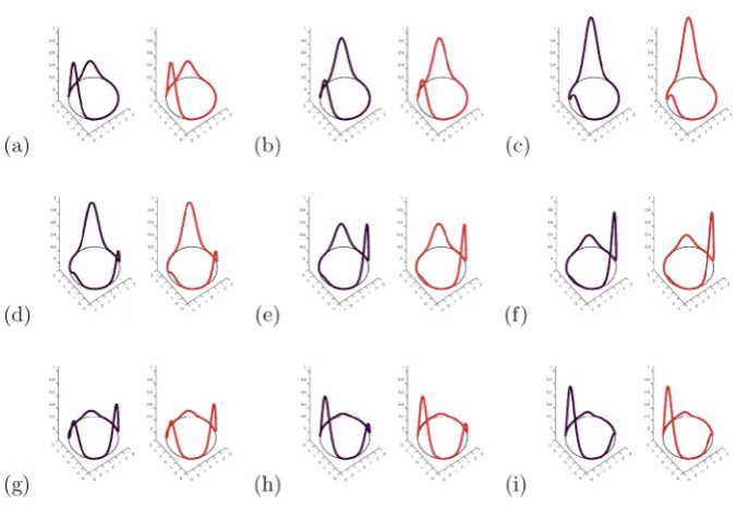
Fig. 1 Original and Reconstructed Time Sequence 1D. Time sequence of excitation of the
one-dimen-sional delay neural field. The original field is shown in black, in red the dynamics based on the delay kernel reconstruction. One cycle of the oscillation is shown at time steps 1, 3, 6, 10, 13, 16, 19, 22, 25, with a step size oft=0.2, in panels (a) to (i)
the whole manifold. The second example instead limits boundary effects by using only small excitations close to the boundary in a two-dimensional neural patch.
Example 1 We start with a simple one-dimensional closed curve or manifold,
respec-tively, embedded in a two-dimensional space. In particular, we study the dynamics of the activity fieldu(r, t )on the boundary∂BR⊂R2of a disk with radiusR, as
dis-played in Fig.1. Here we consider that v=1, and use a simple and smooth delay function forr=(x, y) andr=(x, y)withr, r∈∂BR based on the embedding
intoR2which is defined by
Dr, r:= ˜Dr, r=r−r=x−x2+y−y2, r, r∈∂BR. (53)
This simple sandbox for testing our method hence can be considered as neurons grow-ing on the boundary of a disk, but connectgrow-ing directly through its interior. This is reminiscent of the thin exterior layer of grey matter containing neurons connecting through an interior bulk of white matter containing axons in the brain. However, we point out that this is a different setup from previous studies that superficially appear similar, where the spatial domain instead is a ring with periodic boundary conditions [38,39].
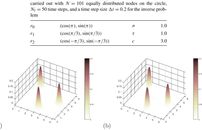
Table 1 Parameter values for Example1. Simulations have been carried out withN=101 equally distributed nodes on the circle,
Nt=50 time steps, and a time step sizet=0.2 for the inverse prob-lem
r0 (cos(π ),sin(π )) σ 1.0
r1 (cos(π/3),sin(π/3)) τ 1.0
r2 (cos(−π/3),sin(−π/3)) c 3.0
Fig. 2 Reconstructed Kernel 1D-Case. For the one-dimensional example the kernel can be visualized as
a two-dimensional scalar functionw(r, r). We display (a) the original and (b) the reconstructed kernel of the one-dimensional delay dynamics shown in Fig.1
rather short temporal window this simple approach is completely sufficient and does not show any deficiencies compared to higher-order methods for the forward prob-lem, as employed for example in [21,28,40].
We first solve the direct problem, i.e., calculate the time-evolution of the excitation fieldu(r, t ). As initial condition, we choose the exponential function
u(r,0)=e−σ|r−r0|2, r∈∂BR. (54)
We prescribe a neural kernel of the form
wr, r=ce−τ|r−r1|2e−τ|r−r0|2+e−τ|r−r2|2e−τ|r−r1|2
+e−τ|r−r0|2e−τ|r−r2|2 (55)
forr, r∈∂BR⊂R2with constantsc >0 andτ >0. The full set of values used for
our simulations are given in Table1. This leads to delayed excitation of areas around three points r0, r1 andr2 equally distributed on a circle, where, with some delay,
the excitation field aroundr0will excite the field aroundr1, the field aroundr1will
excite the field aroundr2and the field aroundr2will excite the field aroundr0again.
The functionf is chosen to be sigmoidal as in equation (6). We have generated a classical oscillator, as can be seen in the snapshots in Fig.1(black curves). Its kernel is visualized in Fig.2(a).
t∈ [0, T]according to equations (30) and (39). Given a discretized version ofu(r, t ) on nodes
r:=
cos
2π· N
,sin
2π·
N
, tk=k·t, (56)
for=0, . . . , Nandk=0, . . . , Nt−1, we calculateφandψaccording to equations
(25) and (26) and then employ the regularization (39) via (42) to solve equation (35) forr∈∂BR. In Fig.2, we compare the original with the reconstructed kernel in the
case where no additional noise is added, carried out withα=0.01 and find a very good agreement between both.
As a test, we employ the reconstructed kernel with the same initial condition to calculate a reconstructed neural fieldurec(r, t )on(r, t )∈∂BR× [0, T]. The original
dynamics is shown in black in Fig.1, based on the kernel (55) visualized in Fig.2(a). The reconstructed dynamics is shown in red in Fig.1, based on the reconstructed kernel visualized in Fig.2(b). A very good agreement between original and recon-structed solution is observed.
Example 2 As a second example, we study oscillating two-dimensional neural field
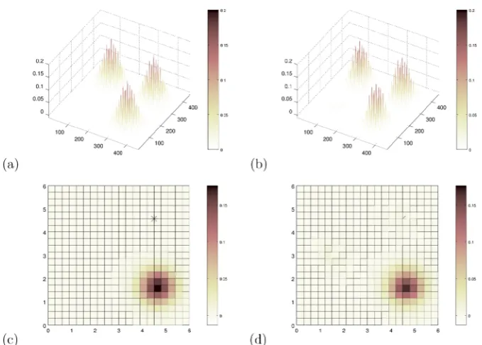
activity. Here, the dimension of the state space is higher withN =21×22=462 spatial elements as shown in Figs.3 and4. Our approach is analogous to the one-dimensional example, but now with 213,444 degrees of freedom for the possible con-nectivity values (see Table2). We first simulate the neural field dynamics based on equation (3) on a neural patch described byΩ:= [a1, b1] × [a2, b2] = [0,6] × [0,6].
Time slices of this dynamical evolution are displayed in Fig.3. The kernel has been chosen to be of a form similar to equation (55), but now with pointsr0,r1andr2in
the two-dimensional neural patch. This leads to an oscillating field in an area around these pointsrj withj=0,1,2. The activation functionf is chosen to be sigmoidal
again. The initial condition is a Gaussian excitation around the pointr0. For our
sim-ple tests, we again employ zeroth or first-order quadrature and Euler’s method to carry out the simulation.
The kernelw(r, r)withr, r∈Ω now lives on a subsetU:=Ω×Ω of a four-dimensional space, sinceΩ is a subset of a two-dimensional patch. Visualization of w(r, r)can be carried out by either fixingr and showing a two-dimensional sur-face plot, or by re-orderingr andr into one-dimensional vectors, so thatw(r, r) can be displayed in full as a two-dimensional surface. The first approach is cho-sen in Fig.4(c), where the white star indicatesr. The second approach is shown in Fig.4(a). Next, we solve the inverse delay neural problem and reconstruct the kernel based on equation (30) regularized as indicated by equations (39) and (42). Again, this is carried out by calculation ofφandψfirst according to equations (25) and (26), then solving equation (35) by regularization via equation (39) with the regularization parameter chosen asα=0.1. This choice leads to a reasonable stability of the recon-structions combined with high reconstruction quality, and it has been chosen by trial and error.
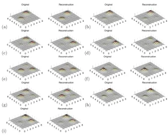
regular-Fig. 3 Original and Reconstructed Time Sequence 2D. Selection of time slices for the two-dimensional
delay neural field. We display time steps 3, 6, 9, 12, 15, 18, 21, 24, 27 witht=0.2 to show one and a half cycles of the oscillation in panels (a) to (i). Each panel shows the original on the left and simulation with the reconstructed kernel on the right
ized reconstruction of the delay neural kernel is not perfect. However, it is working well if the field activity reaches specific parts of the neural environment. Otherwise the reconstruction is just zero due to missing input for the reconstruction equations and the regularization chosen here. The regularization penalizes the distance to the zero kernel function. Therefore, the results clearly demonstrate the feasibility of the method.
5.2 Sensitivity with Respect to Functional Input
In this section we will carry out a numerical sensitivity study of our first example to explore the dependence of the kernel reconstructions on the input functionu. It complements our sensitivity analysis of Sect.4.2.
Fig. 4 Original and Reconstructed Kernel 2D-Case. We display (a) the original and (b) the reconstructed
kernel of the two-dimensional neural delay dynamics shown in Fig.3. The images (c) and (d) show a column of the original and reconstructed kernel, visualizing the connection from the point indicated by the
black star to the rest of the neural patch
Table 2 Parameter values for Example2. Simulations have been car-ried out withN=21×22=462 nodes,Nt=30 time steps with time step sizet=0.2 for the inverse problem. The kernel estima-tion problem has 213,444 degrees of freedom
r0 (1.5,3.0) σ 2.0
r1 (4.5,4.5) τ 1.0
r2 (4.5,1.5) c 2.1
points. The amplitude of the signal is given byε=0.01, which corresponds to noise of 1% added to the measured temporal signal; compare Fig.5.
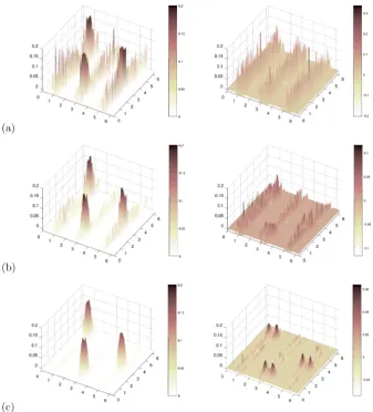
Now, we study reconstructions with different regularization parametersα, where largerα means we regularize in a stronger way, damping the error which comes from the measurement error. Figure6 displays three different choices ofα, where α=1 leads to reasonable reconstructions,α=0.1 shows kernel reconstruction still disturbed by noise, andα=0.01 does not lead to satisfactory reconstructions at all.
Fig. 5 Measured Signal and Measurement Error. In the upper image we display the input signalu(r, t )
independence of the point index of the discretized vectorrand the temporal evolutiont∈ [0, T]. The lower image shows the measurement error which has been added to the signal before a reconstruction has been carried out
6 Conclusions
The purpose of this work is to develop an integral equation approach for kernel re-constructions in delay neural field equations and to study its practical feasibility. We simulate the activity and evolution of a delayed neural field of Amari-type to develop an effective approach to reconstructing the neural connectivity. As a preparation for the inverse problem, this work includes an explicit study of the solvability of the di-rect problem of the delayed neural field equation (3). We provide an easily accessible functional analytic approach based on an integral equation and Banach’s fixed-point theorem.
As our main result, we apply inverse problems techniques to reconstructing the neural kernel assuming that some measurements of the activityu(r, t )are given. We start by formulating a family of integral equations of the first kind. Since kernel re-construction is ill posed, we need regularization to obtain stable solutions. As sta-bilization method we employ the Tikhonov regularization. A sensitivity analysis is carried out, showing that the mapping of the inpututo the regularized kernel recon-struction is Fréchet differentiable. The derivative is explicitly calculated based on the integral equation approach.
Fig. 6 Sensitivity Study of the Influence of Measurement Error. We show reconstruction kernels and the
reconstruction error for 1% noise shown in Fig.5with regularization parametersα=0.01 in (a),α=0.1 in (b) andα=1 in (c). A sufficient reconstruction quality is achieved withα=1
In this work, we assume the delay function D to be given, as it would be the case when the delay is approximately proportional to the distance of the nodes under consideration. IfD is unknown,w is known and u is measured, we can solve in equation (3) for u(r, t −D(r, r)) for allr, r andt. This is still ill posed, since it involves an integral equation of the first kind, but then the determination ofD is reduced to the reconstruction ofDfrom the knowledge ofu(r, t−D(r, r)), which strongly depends on the form of the signalu and conditions we impose on D. If neither the delayDnorw would be given, the kernelKr of operatorVr would be
and observability. In general, the reconstruction of both the kernelwand the delayD is an important nonlinear, far reaching and challenging problem of future research.
In summary, we have developed a stable and efficient approach for the reconstruc-tion of the connectivity in neural systems based on delay neural field equareconstruc-tions. We expect the approach to be extensible to a wide range of field models with delay, and in particular to be highly useful for analyses of experimental data in the domain of computational neuroscience. These methods allow for the reconstruction of the un-derlying ‘synaptic footprint’ of connectivity from available neural activity measure-ments, thus providing a basis for simulation and prediction of real phenomena in the neurosciences.
Acknowledgements The first author would like to thank the Libyan Government which funded her research under the Libyan Embassy Ref No. 10128, Grant 393/12.
Funding Not applicable.
Availability of Data and Materials Data sharing not applicable to this article as no datasets were gen-erated or analysed during the current study. Please contact the author for data requests.
Ethics Approval and Consent to Participate Not applicable.
Competing Interests The authors declare that they have no competing interests.
Consent for Publication Not applicable.
Authors’ Contributions RP, IB and AH, DS and JA interaction on formulation of setup, design of examples, idea and proofreading. JA and RP core proofs, writing and programming. All authors read and approved the final manuscript.
Publisher’s Note
Springer Nature remains neutral with regard to jurisdictional claims in published maps and institutional affiliations.
References
1. Coombes S, beim Graben P, Potthast R, Wright J. Neural fields: theory and applications. Berlin: Springer; 2014.
2. Wilson HR, Cowan JD. Excitatory and inhibitatory interactions in localized populations of model neurons. Biophys J. 1972;12:1–24.
3. Wilson HR, Cowan JD. A mathematical theory of the functional dynamics of cortical and thelamic nervous tissue. Kybernetik. 1973;13:55–80.
4. Amari S. Dynamics of patterns formation in lateral-inhibition type neural fields. Biol Cybern. 1977;27:77–87.
5. Boeree CG. The neurons. General Psychology. 2015. p. 1–6.
6. Bressloff PC, Coombes S. Physics of the extended neuron. Int J Mod Phys B. 1997;11:2343–92. 7. Nogaret A, Meliza CD, Margoliash D, Abarbanel HDI. Automatic construction of predictive neuron
models through large scale assimilation of electrophysiological data. Sci Rep. 2016;6:32749. 8. Gils S, Janssens SG, Kuznetsov Y, Visser S. On local bifurcations in neural field models with
9. Venkov NA. Dynamics of neural field models [PhD thesis]. 2008.
10. Faye G, Faugeras O. Some theoretical and numerical results for delayed neural field equations. Phys-ica D. 2010;239:561–78.
11. Atay FM, Hutt A. Stability and bifurcations in neural fields with finite propagation speed and general connectivity. SIAM J Appl Math. 2005;65(2):644–66.
12. Potthast R, beim Graben P. Existence and properties of solutions for neural field equations. Math Methods Appl Sci. 2010;33:935–49.
13. Venkov NA, Coombes S, Matthews PC. Dynamic instabilities in scalar neural field equations with space-dependent delays. Physica D. 2007;232:1–15.
14. Veltz R, Faugeras O. Stability of the stationary solutions of neural field equations with propagation delays. J Math Neurosci. 2011;1:1.
15. Veltz R, Faugeras O. A center manifold result for delayed neural fields equations. SIAM J Math Anal. 2013;45(3):1527–62.
16. beim Graben P, Potthast R. Inverse problems in dynamic cognitive modeling. Chaos, Interdiscip J Nonlinear Sci. 2009;19:015103.
17. Freitag MA, Potthast RWE. Synergy of inverse problems and data assimilation techniques. In: Large scale inverse problems. Radon series on computational and applied mathematics. 2013. p. 1–54. 18. Potthast R. Inverse problems and data assimilation for brain equations—state and current challenges.
2015.
19. Potthast R. Inverse problems in neural population models. In: Encyclopedia of computational neuro-science. 2013.
20. Potthast R, beim Graben P. Dimensional reduction for the inverse problem of neural field theory. Front Comput Neurosci. 2009;3:17.
21. Nakamura G, Potthast R. Inverse modeling: an introduction to the theory and methods of inverse problems and data assimilation. Bristol: IOP Publishing; 2015.
22. Hutt A. Generalization of the reaction-diffusion, Swift-Hohenberg, and Kuramoto-Sivashinsky equa-tions and effects of finite propagation speeds. Phys Rev E. 2007;75:026214.
23. Coombes S, Venkov N, Shiau L, Bojak I, Liley D, Laing C. Modeling elactrocortical activity through improved local approximations of integral neural field equations. Phys Rev E. 2007;76:051901. 24. Dijkstra K, van Gils SA, Janssens SG. Pitchfork-Hopf bifurcations in 1D neural field models with
transmission delays. Physica D. 2015;297:88–101.
25. Engl HW, Hankle M, Neubauer A. Regularization of inverse problems. Mathematics and its applica-tions. Dordrecht: Springer; 2000.
26. Groetsch CW. Inverse problems in the mathematical sciences. Theory and practice of applied geo-physics series. Wiesbaden: Vieweg; 1993.
27. Kress R. Linear integral equations. Applied mathematical sciences. vol. 82. New York: Springer; 1999.
28. Coombes S, beim Graben P, Potthast R. Tutorial on neural field theory. In: Neural fields: theory and applications. 2014.
29. James MP, Coombes S, Bressloff PC. Effects of quasioctive membrane on multiply periodic travelling waves in integrate-and-fire systems. 2003.
30. Laing CR, Coombes S. The importance of different timings of excitatory and inhibitory pathways in neural field models. 2005.
31. Bojak I, Liley DT. Axonal velocity distributions in neural field equations. PLoS Comput Biol. 2010;6(1):e1000653.
32. Coombes S, Schmidt H. Neural fields with sigmoidal firing rates: approximate solutions. Nottingham e Prints. 2010.
33. Rankin J, Avitabil D, Baladron J, Faye G, Lloyd DJ. Continuation of localised coherent structures in nonlocal neural field equations. 2013.arXiv:1304.7206.
34. Bressloff PC, Kilpatrick ZP. Two-dimensional bumps in piecewise smooth neural fields with synaptic depression. SIAM J Appl Math. 2011;71:379–408.
35. Diekmann O. Delay equations: functional-, complex-, and nonlinear analysis. Berlin: Springer; 1995. 36. Hutt A, Buhry L. Study of gabaergic extra-synaptic tonic inhibition in single neurons and neural
pop-ulations by traversing neural scales: application to propofol-induced anaesthesia. J Comput Neurosci. 2014;37(3):417–37.
38. Hutt A, Bestehorn M, Wennekers T. Pattern formation in intracortical neural fields. Netw Comput Neural Syst. 2003;14:351–68.
39. Wennekers T. Orientation tuning properties of simple cells in area V1 derived from an approximate analysis of nonlinear neural field models. Neural Comput. 2001;13:1721–47.
![Fig. 5 Measured Signal and Measurement Error. In the upper image we display the input signal u(r,t)independence of the point index of the discretized vector r and the temporal evolution t ∈ [0,T ]](https://thumb-us.123doks.com/thumbv2/123dok_us/913230.1589153/20.439.92.347.52.262/measured-signal-measurement-display-independence-discretized-temporal-evolution.webp)