Quantitative methods in neuropathology
Richard A. Armstrong
Vision Sciences, Aston University, Birmingham, UK
Folia Neuropathol 2010; 48 (4): 217-230
A b s t r a c t
The last decade has seen a considerable increase in the application of quantitative methods in the study of histo-logical sections of brain tissue and especially in the study of neurodegenerative disease. These disorders are charac-terised by the deposition and aggregation of abnormal or misfolded proteins in the form of extracellular protein deposits such as senile plaques (SP) and intracellular inclusions such as neurofibrillary tangles (NFT). Quantification of brain lesions and studying the relationships between lesions and normal anatomical features of the brain, includ-ing neurons, glial cells, and blood vessels, has become an important method of elucidatinclud-ing disease pathogenesis. This review describes methods for quantifying the abundance of a histological feature such as density, frequency, and ‘load’ and the sampling methods by which quantitative measures can be obtained including plot/quadrat sampling, transect sampling, and the point-quarter method. In addition, methods for determining the spatial pattern of a his-tological feature, i.e., whether the feature is distributed at random, regularly, or is aggregated into clusters, are described. These methods include the use of the Poisson and binomial distributions, pattern analysis by regression, Fourier analysis, and methods based on mapped point patterns. Finally, the statistical methods available for study-ing the degree of spatial correlation between pathological lesions and neurons, glial cells, and blood vessels are described.
Key words: neurodegenerative disorders, quantitative measurements, abundance, sampling methods, spatial pat-tern, spatial correlation.
Communicating author:
Dr R.A. Armstrong, Vision Sciences, Aston University, Birmingham B4 7ET, UK, phone 0121-359-3611, fax 0121-333-4220, e-mail: [email protected]
Introduction
The last decade has seen a considerable increase in the application of methods designed to quantify features visible in histological sections of brain tissue [6,9,10]. In addition, image analysis systems have enabled images to be captured and enhanced on a com puter screen so that histological features can be quantified more rapidly and objectively [70,71].
Many quantifiable histological objects are visible in thin sections of brain tissue and include the cell
lesions are important both in the pathological diag-nosis of disorders [6] and in studies of disease patho-genesis [7,9,10].
This article reviews the various methods available for quantifying features in thin histological sections and includes a discussion of: 1) the sampling methods by which quantitative measures can be obtained, 2) methods of quantifying the abundance of a histo-logical feature, 3) methods for determining the spa-tial pattern of a feature, i.e., whether the object is dis-tributed at random, regularly or is aggregated into clusters, and 4) methods for measuring the degree of spatial correlation between pathological lesions and normal anatomical features of the brain such as neu-rons, glial cells, and blood vessels.
Quantifying histological features in 2D
For objects in brain tissue such as cells or patho-logical features, one does not see the projection of the whole object but a sectional profile, the shape and size of which depend on where the individual object is cut. In addition, objects are hit by sectioning planes with a probability proportional to their tangent diameter orthogonal to the section [10]. Hence, large objects are cut by many planes while small objects are hit more rarely. The sectional profiles of objects revealed in 2D sections are therefore not a random sample of such objects in a volume of tissue and the parameters estimated by analysing their abundance
and distribution are not valid estimates of their true distribution in 3D. In most circumstances, studies will be carried out on 2D sections taken from a complex 3D structure, and without serial sectioning, 3D micro-scopic methods such as confocal scanning laser microscopy, or the optical dissector method [60], 3D inference will not be possible. Brain tissue has a complex cytoarchitecture, the cerebral cortex, for example, having a laminar structure in which the cells of origin or axon terminals of specific anatomical pro-jections are located within particular laminae [37]. In addition, the cells of origin of the projections that connect different gyri of the cerebral cortex are arranged in clusters that are regularly arranged paral-lel to the pia mater [37]. Hence, it is often useful to study spatial distributions in brain in thin strips of tis-sue in relation to tistis-sue landmarks, e.g., parallel to the pia mater or across the laminae from pia mater to white matter [24].
Sampling methods for obtaining
quantitative measurements
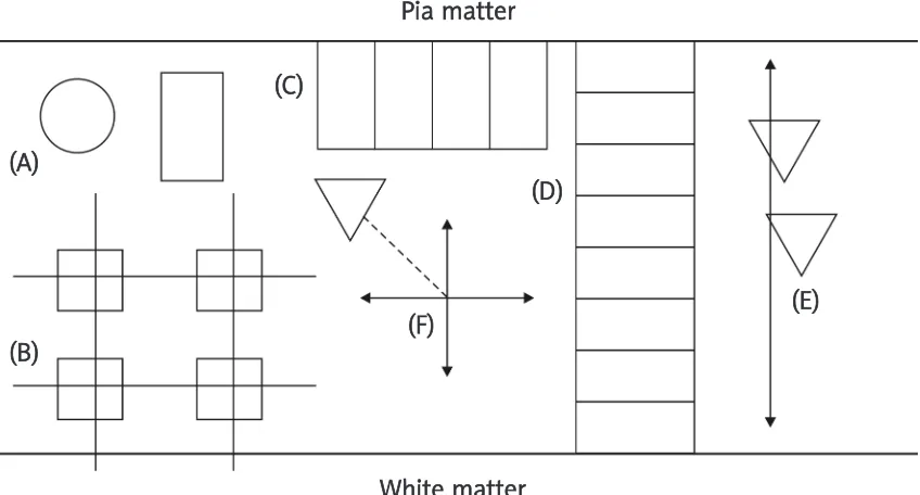
A number of sampling methods can be employed to obtain a quantitative measure from a histological section (Fig. 2). The most commonly used methods are plot or quadrat sampling, transect sampling, and point-quarter sampling [6].
Plot/Quadrat sampling
Sampling with 2D plots of defined dimension is the most commonly used procedure (Fig. 2A). The plots (sample fields) may be rectangular, square, or circular in shape, although the rectangular plot is often regarded as the most efficient method of sam-pling a 2D surface [28]. Positioning the plot relative to the section may be determined by overlaying a grid or other systematic method (Fig. 2B) or by a standard random procedure to minimize bias [34].
Transect sampling
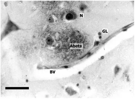
Transect sampling is useful when there is a sys-tematic change in the abundance of an object in a particular direction. A common method of sampling the cerebral cortex, for example, is the use of con-tiguous, rectangular sample fields that follow the contours of the sulci and gyri (Fig. 2C) [5]. This sam-pling regime is useful in studying the changes in abundance of pathological lesions that may occur Fig. 1. Histological features visible in a thin
sec-tion of brain tissue taken from the temporal
cor-tex in a case of Alzheimer’s disease (AD) (β
-amy-loid immunohistochemistry, haematoxylin; bar
= 25 µm).
along the cortex parallel to the pia mater. In addition, the method has been extensively used to study changes across the laminae of the cortex (Fig. 2D) [21,37,41,44].
Two types of transect sampling can be used. First, in a ‘belt transect’ (Fig. 2D), a strip of tissue is sam-pled in which all histological features of interest are counted or measured, and this is the method most commonly employed [5,6]. If the transect is divided into contiguous plots, data for all plots can be used to compute a quantitative measure. An example of the use of the ‘belt transect’ method to study the laminar distribution of the vacuoles and PrPsc deposits in a case of the variant form of CJD (vCJD) is shown in Fig. 3. The distribution of the vacuoles across the cor-tex is essentially bimodal with peaks of density in the upper and lower cortex while the PrPsc deposits are distributed either in the superficial cortical layers or in the lower cortical laminae [24]. This distribution suggests that the cells of origin of the feedforward and/or feedback cortico-cortical pathways may be affected in the pathology of CJD [24]. Secondly, in the more rarely used line-intercept method (Fig. 2E), data are tabulated on the basis of the features that
inter-1000
800
600
400
200
0
0 5 10 15 20 25 30 35
Fig. 3. Laminar distribution of the vacuoles and
prion protein (PrPsc) deposits in the occipital
cortex in a case of variant Creutzfeldt-Jakob
dis-ease (vCJD) (data from Armstrong et al. 2002).
The fitted curves are third and fourth-order polynomials fitted to the florid deposits and vacuoles respectively.
Density (50 × 250 µm field)
Florid PrP deposits
Vacoulation
Fig. 2. Sampling methods by which quantitative estimates of histological features can be obtained: A) plot sampling (circular or rectangular plot), B) grid sampling, C) transect sampling (parallel to pia mater), D) transect sampling (across cortical laminae), E) the line-intercept method, F) point-quarter sampling.
(A)
(B)
(F)
(C)
(D)
(E)
Pia matter
White matter
Distance fr
sect a straight line that cuts across an area to be sampled.
Point-quarter sampling
Plot-based methods may be laborious and time-consuming and the results are often dependent on the size, shape, and the number of the plots sampled [1]. By contrast ‘plotless’ sampling has the advantage of not demarcating sampling areas of a certain size or shape. Plotless methods are sensitive, however, to departures from a random distribution of individual objects, especially if the sample size is small [28]. The plotless sampling method of choice is the ‘point-quar-ter method’ (Fig. 2F) and is regarded as superior to other plotless methods such as the nearest-neigh-bour method [6].
To employ the point-quarter method, a number of points are established in the area to be sampled. These points may be randomly distributed through-out the whole area or randomly located along a belt transect, e.g., parallel to the pia mater. Each point is considered to be the centre of four compass direc-tions dividing the area into four quarters. In each quarter, the distance from the centre point to the nearest object of interest is measured: four objects measured to each point. Data on the mean density of an object per unit of area, frequency, and coverage can all be obtained by this method [6].
Quantifying the abundance of histological
features
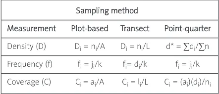
The various methods of expressing the abundance of a histological feature together with the relevant statistics are shown in Table I.
Density
The term ‘abundance’ (N) describes the number of individual lesions in a given area of the section, whereas density (D) is N expressed per unit of area or volume (Table I). For example, if there are 100 individ-ual lesions in an area of 2.5 mm2of tissue then densi-ty is 40 lesions per mm2.
There are two problems in obtaining an accurate density measurement of a feature in histological sec-tions. First, it may be difficult to define an appropriate area in which the density measurement is relevant. A pathological lesion, for example, may develop in relation to the cells of origin of a specific cortical pro-jection and be confined to specific cortical laminae [37]. Hence, NFT in AD are frequently found in greater abundance in laminae II and III [12,44,57] while LB in dementia with Lewy bodies (DLB) are found largely in the lower cortical laminae [16]. Hence, density measu-rements may need to be restricted to particular lami-nae rather than involve the whole of the cortical pro-file. Second, it may be difficult to define what constitutes an individual lesion [34]. Neurons [42], glial cells [56] and inclusions such as NFT in AD [27,33] and progressive supranuclear palsy (PSP) [45], LB in DLB [61,63] and PB in Pick’s disease (PD) [18] are rela-tively discrete objects and can be counted successful-ly. By contrast, it is more difficult to define the bound-aries of aggregated protein deposits such as the diffuse-type SP in AD [38] or the synaptic-type PrPsc deposits observed in sporadic CJD (sCJD) [21,65]. In circumstances where it is impossible to define an ‘individual’, alternative measures of abundance such as ‘coverage’ or ‘load’ can be used.
The use of density measurements in quantifying PrPsc deposition in various brain areas in vCJD is shown in Fig. 4. The data are displayed as a histogram with brain region as a categorical variable (X axis) and mean density (averaged over cases) with appropriate standard errors (SE) or confidence intervals (CI) as the Y axis. The data reveal the relatively low densities of PrPscdeposits in the hippocampus and dentate gyrus compared with the neocortex and the high density of uncored (‘diffuse’) deposits in the cerebellum.
Frequency
To determine the frequency of a feature, the num-ber of samples in which a particular type of object is present is counted, e.g., if the object occurred in 7/10 samples, the probability of finding it in an area of
tis-Sampling method
Measurement Plot-based Transect Point-quarter
Density (D) Di= ni/A Di= ni/L d* = ∑di/∑n
Frequency (f) fi= ji/k fi= di/k fi= ji/k
Coverage (C) Ci = ai/A Ci= li/L Ci= (ai)(di)/ni
Table I. Quantitative measurements for differ-ent sampling methods
sue would be 0.7 and its frequency 70% (Table I). Fre-quency measurements provide a rapid method of indicating the abundance of an object in a tissue section. Frequency estimates are, however, highly dependent on the size and shape of the plots used. If plots are too large, then it is certain that all types of object, common or rare, will be found in a plot, whereas if the plots are too small, then a less com-mon object may be insufficiently recorded. In addi-tion, frequency measurements are very sensitive to the distribution pattern of individual lesions, i.e., whether the lesion is distributed at random, regularly, or is aggregated into clusters [1,3]. Many types of lesion in neurodegenerative disorders exhibit a clus-tered or aggregated distribution [22] and sample plots of different size may be necessary to estimate their frequency [1].
Cover (mass or load)
Mass or load is the amount of a lesion present in the tissue and may be appropriate when measuring less circumscribed lesions such as diffuse Aβor PrPsc deposits (Table I) [34]. Image analysis systems fre-quently provide estimates of this type of measure-ment by measuring ‘coverage’. Cover is the propor-tion of the area of the sample that is occupied by a lesion in relation to the total area in which the lesion could occur. This method was used to quantify the percentage of tissue occupied by spongiform change in CJD [49,68,69]. Coverage values can also be obtained by using a sample field divided into a grid and counting the number of times the points of inter-section of the grid overlay the object under study. This method has been used to estimate the abundance of diffuse ‘synaptic-type’ PrPsc deposits in sCJD (Fig. 5) [21], Aβload in AD [30,34], and blood vessel profiles in AD [11]. Load is sometimes considered a more useful measure than absolute density in the study of neu-rodegenerative disorders since it may be more close-ly correlated with clinical symptoms.
Semi-quantitative scores
A rapid method of describing the abundance of a lesion in a tissue section is to assign a subjective assessment of abundance. For example, the “Consor-tium to Establish a Registry for Alzheimer’s disease” (CERAD) criteria for the clinico-pathological diagnosis of AD [54] scores the abundance of senile plaques (SP) on a four-point scale, viz., none, sparse,
moder-ate, or frequent. Such a scale can be used not only for diagnostic purposes but also for large-scale studies of many patients and brain areas in which it may not be
15
10
5
0
FC PC OC ITG PHG HC DG CB
Mean n
umber of conta
cts
Sporadic CJD: PrP deposits
Fig. 5. Estimation of the ‘coverage’ of the
synap-tic-type PrPscdeposits in various brain regions,
averaged over cases, in sporadic Creutzfeldt-Jakob disease (sCJD). Error bars represent stan-dard errors of the mean.
FC – frontal cortex, PC – parietal cortex, OC – occipital cor-tex, ITG – inferior temporal gyrus, PHG – parahippocampal gyrus, HC – CA1/2 sectors of hippocampus, DG – dentate gyrus molecular layer, CB – cerebellum molecular layer
4
3
2
1
0
FC PC OC ITG PHG HC DG CB
Mean density (50 × 250 µm f
ie
ld)
Uncored
Amyloid-type
Fig. 4. The density of PrPsc deposits in various
brain regions, averaged over cases, in variant Creutzfeldt-Jakob disease (vCJD). Error bars rep-resent standard errors of the mean.
practicable to obtain more accurate density measure-ments [50]. This method was used to study the degree of neuropathological heterogeneity within a group of 80 cases of AD [20]. The limitations of semi-quantitative scores, however, are the large unconscious error of judgment and the consequent high between-observer variability of the scores.
Measuring spatial pattern in a tissue
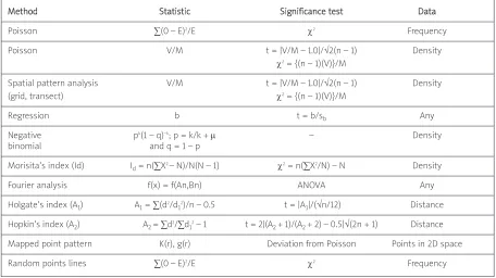
Measuring the spatial pattern of an object, i.e., whether the object is distributed at random, regular-ly, or forms clusters, may provide more information than a simple estimate of abundance [9,10]. Hence, the spatial pattern of a pathological lesion such as NFT or LB may reflect the degeneration of underlying neuroanatomical structures, and hence may be use-ful in determining lesion pathogenesis [1]. Various methods of measuring spatial pattern can be used and are summarized in Table II.
The Poisson distribution
Methods based on the Poisson distribution are the most commonly used to measure spatial pattern
[9,57]. Any type of plot sampling can be used to fit the Poisson distribution to data, including randomly dis-tributed plots, a transect of contiguous plots, or a grid of plots. If the distribution of individuals is random then the probability (P) that the plots contain 0, 1, 2, 3, ..., n, individuals is given by the Poisson distribution [1]. In a Poisson distribution, the variance (V) is equal to the mean (M), and hence the V/M ratio is unity. The V/M ratio (Table II) is an index of spatial pattern, uni-form distributions having a V/M ratio less than unity and clustered distributions greater than unity. The significance of departure of the V/M ratio from unity can be tested by a ‘t’ test or by a chi-square (χ2) test [28].
A disadvantage of the Poisson method is that the results are markedly affected by plot size. To over-come this problem, if contiguous samples or grid-sampling is used, quantitative measures in adjacent plots can be added together successively to provide the data for increasing plot sizes up to a size limited by the length of the strip sampled [1,3]. V/M is plotted at each field size and the resulting graph will indicate whether the clusters of lesions were regularly or ran-domly distributed and the scale at which clustering is
Method Statistic Significance test Data
Poisson ∑(0 – E)2/E χ2 Frequency
Poisson V/M t = |V/M – 1.0|/√2(n – 1) Density
χ2= {(n – 1)(V)}/M
Spatial pattern analysis V/M t = |V/M – 1.0|/√2(n – 1) Density
(grid, transect) χ2= {(n – 1)(V)}/M
Regression b t = b/sb Any
Negative pk(1 – q)–k; p = k/k + µ – Density
binomial and q = 1 – p
Morisita’s index (Id) Id= n(∑X2 – N)/N(N – 1) χ2= n(∑X2/N) – N Density
Fourier analysis f(x) = f(An,Bn) ANOVA Any
Holgate’s index (A1) A1= ∑(d2/d12)/n – 0.5 t = |A1|/(√n/12) Distance
Hopkin’s index (A2) A2 = ∑d2/∑d12– 1 t = 2|(A2 + 1)/(A2 + 2) – 0.5|√(2n + 1) Distance
Mapped point pattern K(r), g(r) Deviation from Poisson Points in 2D space
Random points lines ∑(0 – E)2/E χ2 Frequency Table II. Formulae and significance tests for studying spatial pattern in histological sections
evident. A peak indicates regularly distributed clus-ters of lesions, while the field size corresponding to the peak is an indication of the mean cluster size. This method has been used to study the spatial pattern of lesions in several neurodegenerative diseases, includ-ing Aβdeposits and NFT in AD [2], LB in DLB [17], PB in Pick’s disease (PD) [18], and glial cytoplasmic inclu-sions (GCI) (Papp-Lantos leinclu-sions) in multiple system atrophy (MSA) [25].
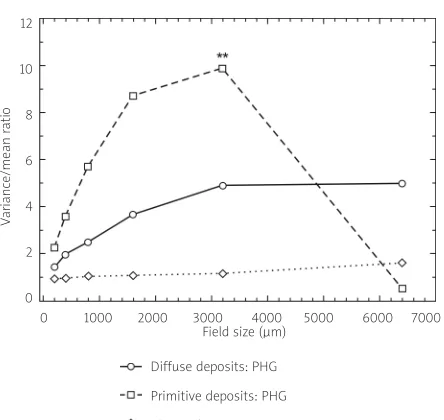
An example of the use of this method to study the spatial pattern of the diffuse, primitive, and clas-sic types of Aβdeposit in the temporal lobe of a case of AD is shown in Fig. 6 [13]. Contiguous samples (N= 64), 200 × 1000µm in size, were arranged along cortical laminae II and III in a belt transect, the short-er dimension of the sample field parallel to the edge of the pia mater. The data show: 1) that the V/M ratio of the diffuse deposits increased with field size with-out reaching a peak, suggesting the presence of large clusters of diffuse deposits of at least 6400 µm in diameter; 2) the V/M of the primitive deposits increased with field size, indicating clustering of the deposits, and reached a peak at field size 3200 µm, after which V/M declined, suggesting the presence of clusters of primitive deposits approximately 3200 µm in diameter and regularly distributed parallel to the pia mater; and 3) the V/M ratio of the classic deposits was approximately unity at all field sizes, suggesting a random distribution. The type of spatial pattern exhibited by the primitive deposits is commonly seen in several neurodegenerative disorders [22] and has led to the conclusion that the lesions developed as a result of the degeneration of specific anatomical pathways [10,35].
Spatial pattern analysis by regression
A disadvantage of the V/M method is that it is based on the Poisson distribution and can only be applied to data in the form of counts or frequencies. Non-density data such as area of an object or protein ‘load’ therefore cannot be analysed using this method [1,3]. An alternative method of analysis, based on a linear regression model, has been described [1,72] and can be used on any quantitative measure obtained from the plots. As in the V/M method, a measure of a histological feature is made in a series of contiguous plots arranged in a belt tran-sect. This type of analysis is based on the observation that if lesions are distributed in discrete clusters and
regularly distributed along the transect, the amount of a lesion in adjacent plots (comprising the X and Y variables of the analysis) will be high in both plots if they are sampling a cluster and low if they sample an intervening space. If the spacing between the plots is increased (e.g., if X and Y are the first and third fields, second and fourth fields, etc.), the probability increas-es that there will be pairs of valuincreas-es such that one member of the pair will fall within a cluster and the other within an adjacent space. Hence, the degree of positive correlation between the sample pairs should decrease as the spacing increases. In theory, the correlation between sample pairs should become signi -ficantly negative when the spacing between the X and Y variables corresponds to the average size of the clusters. Moreover, when the spacing between the X and Y variables corresponds to the distance between regularly distributed clusters, a significant positive correlation should be found. This occurs because the pairs of values are now so widely spaced that they sample adjacent clusters or spaces. Hence, linear regression coefficients (β sample coefficient ‘b’) (Table II) are calculated between pairs of adjacent values and then with increasing degrees of separa-tion (i.e., separated by 1, 2, 3, 4, 5, …, nunits). The reg
-Fig. 6. Spatial pattern analysis of the diffuse, primitive, and classic deposits in the temporal neocortex in a case of Alzheimer’s disease (**represent significant V/M peaks) (data from Arm strong 2010).
12
10
8
6
4
2
0
0 1000 2000 3000 4000 5000 6000 7000 Field size (µm)
V
a
riance/mean r
ati
o
Diffuse deposits: PHG
Primitive deposits: PHG
ression coefficient is plotted as a function of the degree of separation of the pairs of samples. A ‘t’ test of the regression coefficient [66] can be used to test the significance of the positive and negative peaks.
The negative binomial distribution
The negative binomial distribution can be fitted to a variety of clustered patterns and may give a more accurate estimate of the intensity of clustering. The negative binomial is a two-parameter distribution defined by the mean density of individuals (µ) and the binomial exponent ‘k’ (Table II). The value of ‘k’ is generally between 0.5 and 3.0 and decreases as the degree of clustering increases, and hence the recipro-cal of ‘k’ is used as an index of the degree of cluster-ing. The procedure for fitting the negative binomial to data is given by Cox [32]. Essentially, any sample information about the numbers of histological fea-tures can be analysed as long as the mean number of individuals per sample is low and plot size is adjusted to reflect this limitation. Data are grouped as a fre-quency distribution to show the number of samples (f) containing various numbers of individuals (X). The mean number of individuals per plot is then calculat-ed and ‘k’ estimated by an iterative procedure. The expected frequencies of samples containing various numbers of individuals can then be calculated and compared with the observed distribution to test whether the negative binomial is an adequate fit to the data. If the data do fit the distribution, then 1/k will estimate the intensity of aggregation.
Morisita’s index of dispersion
Morisita’s index of dispersion [55] is an alternative method of determining clustering which has the addi-tional advantage that the index is unaltered if objects have disappeared at random from the original clus-ters. This may be especially relevant in the analysis of neuronal populations since cell losses frequently occur as a consequence of disease. Morisita’s index of clus-tering (Id) (Table I) is unity for a random distribution, zero for a perfectly uniform distribution, and equal to ‘n’ when individuals are maximally aggregated. The nificance of Idcan be tested by aχ2test (Table II).
Fourier analysis
Bruce et al. [29] described a method of determin-ing the spatial pattern of histological features across
the different laminae of the cerebral cortex. The data comprised measurements of the amount or ‘load’ of
β-amyloid at different levels in the cortex. A Fourier series was calculated as a series of harmonic compo-nents (Table II) and analysis of variance (ANOVA) was used to determine the presence of significant har-monics. If no significant harmonics were found, this indicates that the distribution was random. The num-ber of significant harmonics may indicate the numnum-ber of clusters present and the curve of best fit can be used to describe the ‘grain’ of the pattern. Significant harmonics were detected in the parahippocampal gyrus (PHG), suggesting the presence of clustering of Aβ deposits in relation to particular laminae [29]. A variation of this method has been applied recently to the spatial distribution of the diffuse, primitive, and classic Aβ deposits in the temporal lobe in AD [14]. It was concluded that Aβdeposits exhibit com-plex sinusoidal fluctuations in density in the temporal lobe in AD, that the fluctuations in Aβ deposition may reflect the formation of Aβdeposits in relation to the modular and vascular structure of the cortex, and that Fourier analysis may be a useful statistical method for studying the patterns of Aβdeposition both in AD and in transgenic models of disease.
Plotless methods of determining spatial
pattern
Spatial pattern can also be determined but with-out the necessity for plot sampling. In Holgate’s method [9,46], a number of randomly selected points (‘n’ at least 50) are superimposed over the area of the section to be sampled. From each point, the dis-tance to the nearest object of interest (d) is meas-ured and the distance to the second nearest object (d1). The index of aggregation (A1) (Table II) is zero for a random distribution, greater than zero for a conta-gious distribution, and less than zero for a uniform distribution.
Methods based on mapped point
patterns
In many circumstances, histological features can be considered to be points in a plane, and therefore can be studied as a 2D point pattern. Hence, some methods measure the distribution of a point pattern, i.e., a spatial point process (SPP) in which the objects consist of a series of mapped point locations within a defined study region.
A number of methods have been used to quantify the characteristics of SPPs [36,39,62]. Ripley’s K-func-tion, K(r)[26,62,64], is a method of analysing com-pletely mapped SPPs in a plane. K(r)as defined by Ripley [62] is the expected number of further points that are within a given distance ‘r’ of an arbitrary point of the process divided by the intensity of the processλ, i.e., the mean number of points per unit of area. K(r)describes the characteristics of a point pat-tern at different distance scales, which many nearest-neighbour based methods do not. For a few SPPs, the expected number of points can be calculated. One of the most common procedures is to test the null hypothesis that objects are distributed at random using the Poisson distribution as described above [62]. For a Poisson distribution, K(r)is the area of a circle of radius r, i.e., K(r)= Πr2, K(r)< Πr2indicates inhibition or regularity, andK(r)> Πr2indicates the presence of heterogeneity or clustering [62]. The K-function can be used to summarize a point pattern, to test hypotheses about the pattern, to estimate parame-ters, or to fit models. In addition, bivariate and multi-variate point patterns can be analysed to investigate the relationships between two or more different point patterns [31].
Diggle et al. [40] used K(r)and other second-order statistics, such as the pair correlation function g(r), to study the spatial distributions of pyramidal neurons in the cingulate cortex of human subjects in three patient groups, viz., normal, schizoaffective, and schi -zophrenic individuals. The objective was to identify anatomical differences between the three groups of patients, and the study subsequently demonstrated abnormal spatial patterns of neurons in the schizo-phrenic patients. These methods have also used been used to characterize neuronal and glial cytoarchitec-ture in the prefrontal cortex in major depressive dis-order (MDD), schizophrenia, and bipolar disdis-order [31].
Methods based on random test points
and random test lines
Some of the methods of measuring spatial pat-tern rely on the use of random points or lines. In immunoelectron microscopy, for example, gold parti-cles are often used to bind to antigens associated with various structures within the cell such as organelles or membranes [58]. The question may arise as to whether the distribution of the labelled particles attached to the organelles or other struc-tures is random [43]. The number of labelled particles lying on each type of identified organelle is used to generate an observed frequency distribution (O). By randomly superimposing a grid of test points on the same cell profiles, the frequency with which the points of intersection of the grid overlie the orga -nelles is determined. This provides an expected dis-tribution of contacts because random points hit organelles on sections with probabilities determined by the area of the organelle. A similar approach employing lines can be used to test the association between immunogold labelling and cell membranes [53]. For a random distribution, the ratio of observed to expected frequencies will be unity and deviations of the observed from the expected distribution can be tested using χ2[53]. Test points and lines, superim-posed over the image, can also be used to study spa-tial relationships over a range of length scales and to calculate K(r)and g(r)[51-53,60,67].
Measuring spatial correlation
In many neurodegenerative diseases, there may be more than one type of lesion present in the tissue, e.g., AD is defined by the presence of both Aβdeposits and NFT [8] and CJD by the presence of vacuolation (‘spongi-form change’) and PrPscdeposits [23]. The degree of spa-tial association between the various lesions and between lesions and normal features of the brain such as neurons, glial cells, and blood vessels may be useful information in elucidating the pathogenesis of the dis-order [7]. Several methods are available for testing whether different features are spatially correlated and include methods based on contingency tables and on grids or transects of contiguous plots (Table III).
The coefficient of association (C
7)
data arranged in a 2 × 2 contingency table. A number of plots are located at random within a tissue section and the presence or absence of two histological fea-tures (A,B) is recorded within each sample unit. From the contingency table, a coefficient of association (C7) can be calculated which varies from +1, when the maximum possible co-occurrence is present, to –1, the minimum possible co-occurrence. Values close to zero indicate that the frequencies of the two features are close to those that would be expected to occur by chance. The actual calculation of C7 depends on the relationships between the numerical values in the contingency table and are dependent on first, whether the product of the joint presences and joint absences (ad) is greater or less than the product of samples which contain one feature alone (cb), and second, on the relative magnitude of ‘c’ and ‘b’ and ‘a’ and ‘d’ [5]. This method was used by Armstrong [8] to determine the degree of spatial association between SP and NFT in AD. In the brain regions analysed, val-ues of C7were in the range –0.31 to +0.32, but a sta-tistically significant spatial association between SP and NFT was present in only 8/39 (21%) regions. The degree of spatial association between SP and NFT was similar in different brain regions and did not vary with apolipoprotein genotype of the patient. How-ever, the magnitude of C7in a region was posi-tively correlated with the density of the NFT and with the total density of SP and NFT but not with the den-sity of SP alone. It was concluded that there was little
evidence that SP and NFT were spatially associated except in brain areas with high densities of lesions. The data support the hypothesis that SP and NFT are distributed relatively independently in the cerebral cortex and hippocampus in AD [15].
Chi-square in 2 × 2 contingency tables
An alternative approach to the statistic C7is to cal-culate χ2 from the frequencies in the contingency table. Chi-square is a test of the null hypothesis that the two histological features are distributed indepen -dently. Since the χ2distribution is continuous and is being used in this case to approximate to a discrete distribution, it is necessary to make a ‘correction for continuity’ (‘Yates’ correction) [59] (Table III) and this statistic is usually given the symbol X2.
Correlation between more than two
histological features
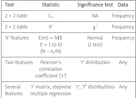
It may be necessary to explore the joint occur-rences of more than two histological features, e.g., whether the different morphological types of SP (dif-fuse, primitive, classic, and compact plaques) occur together more often than chance would suggest [4,38]. With more than two histological features, the contingency tables become more complex, but it is still possible to determine whether the features as a whole are positively associated (Table II). A group of ‘k’ histological features will be positively associated as a whole if an unexpectedly large number of plots contain representatives of all of them. Hence, it is possible to test the difference between the observed and expected frequencies for the class defined by the joint occurrences of all the features [59]. Similarly, it would be possible to test the number of units con-taining no individuals of any of the histological fea-tures or ‘empty’ plots (M).
Correlation based on contiguous plots
If the plots are arranged in a grid or as a transect of contiguous plots, it is possible to study the effect of plot size and distance on the nature of the correlation between two features and to establish the scale at which the correlation is most evident [23]. For exam-ple, a significant correlation between SP in AD and blood vessels using small plots approximating to the size of individual plaques would suggest a close rela-tionship between the two features. By contrast, if a
cor-Test Statistic Significance test Data
2 × 2 table C7 NA Frequency
2 × 2 table X2 χ2 Frequency
‘k’features E(m) = NΠ Normal Frequency (I = 1 to k) (ztest)
(N – ni/N)
Two features Pearson’s ‘r’ distribution Any correlation
coefficient (‘r’)
Several ‘r’ matrix, stepwise ‘r’, ‘F’ distributions Any features multiple regression
Table III. Formulae and significance tests for studying correlation between features in histo-logical sections
NA – not available; C7– coefficient of association, χ2– chi-square, X2–
chi-square corrected for continuity, E(m) – expected number of empty plots, N – total frequency, ni– number of plots with the ‘ith’ histological feature,
relation was only present in much larger plots, then it could be fortuitous, resulting from the abundance and widespread distribution of the plaques and blood vessels in the AD brain.
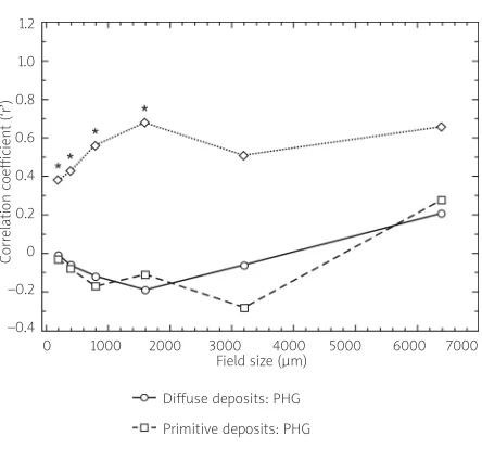
This aspect of spatial pattern analysis can be studied by the use of a correlation coefficient. A quan-titative measure such as density, coverage, or ‘load’ is obtained for two histological features in a series of plots arranged contiguously in a belt transect. Quan-titative measurements in adjacent plots are added together successively to provide data for larger plot sizes, e.g., two unit blocks, four unit blocks etc., up to a size limited by the length of the transect. Pearson’s correlation coefficient (‘r’) or a non-parametric lation coefficient can be used to determine the corre-lation at each field size. An example of the use of this method in AD to study the spatial correlation bet -ween the diffuse type of Aβdeposits and blood ves-sels is shown in Fig. 7 [19]. There is a significant spa-tial correlation between the classic deposits and blood vessels at field sizes from 200 to 1600 µm, indi-cating a close spatial relationship at distances less than 1600 µm. By contrast, the diffuse and primitive deposits were not significantly correlated with blood vessels at any field size. These data suggest that blood vessels are specifically involved in the forma-tion of the classic deposits in AD and that other fac-tors may be involved in the formation of the diffuse and primitive deposits [4]. The spatial correlation between several histological features can be studied using a correlation analysis and stepwise multiple regression [7].
Discussion and conclusions
Quantitative analysis of thin sections of brain tis-sue is increasingly important both in the diagnosis of neurodegenerative disease and in studies of disease pathogenesis [1,6,9,10]. Hence, application of appro-priate sampling strategies, quantitative measures of abundance, and data analysis methods are becoming an essential part of neuropathological methodology.
A quantitative measurement needs to be relevant to the specific objectives of a study. Frequency mea-surements or semi-quantitative scores often provide a quick and easy method of indicating the abundance of a lesion in the tissue, but lack precision, and the former are highly dependent on the size and shape of the plots. They are therefore useful in preliminary quantitative surveys of cases and may provide
sufficiently accurate data for a largescale study of hete -rogeneity within a particular disorder using a method such as principal component analysis (PCA) [20]. Den-sity measurements, by contrast, provide the most reliable measure of lesion abundance, and are essen-tial for studying spaessen-tial patterns and spaessen-tial correla-tions between different types of histological feature, but the data are time-consuming to obtain for large numbers of patients or cases. In some circumstances, individual lesions cannot be identified and coverage or load may be a more appropriate measure than density.
A number of different methods are available for measuring the spatial pattern of a histological feature [1,3]. If the objective is simply to determine whether a feature is distributed at random in a tissue, then one of the methods based on the V/M ratio could be used. A major disadvantage of the simpler methods is that spatial patterns are markedly affected by the size and shape of the plots. In addition, brain lesions often exhibit a complex spatial pattern in brain tissue [22] with small clusters of lesions regularly distributed parallel to the tissue boundary and further aggregated into larger scale clusters. In these cases, analyses based on grids or transects are essential in providing information on the different scales of clustering
pre-Fig. 7. Spatial correlations between the diffuse,
primitive, and classic β-amyloid (Aβ) deposits
and associated cerebral blood vessels in the temporal cortex of a case of Alzheimer’s disease (*significant Pearson’s correlation coefficient at
P< 0.05) (data from Armstrong 2010).
1.2
1.0
0.8
0.6
0.4
0.2
0
–0.2
–0.4
0 1000 2000 3000 4000 5000 6000 7000 Field size (µm)
Corr
e
lati
on co
eff
icient (‘r’)
Diffuse deposits: PHG
Primitive deposits: PHG
sent. An alternative strategy is to use a plotless method of sampling that involves determining the dis-tance between an object and its nearest neighbour of the same type. A problem in applying these methods is that an object nearest to a random point cannot be taken as a ‘randomly chosen’ member of the popula-tion as this would result in a biased sample [59]. Hence, a random individual would have to be selected from the population as a whole. This would require a com-plete census of the population and would be a very dif-ficult task if the feature was especially numerous.
Methods determining the degree of correlation between two histological features fall into two distinct categories, viz., those based on contingency tables in which the presence and absence of lesions are analysed, and more quantitative methods which use transects or grids of contiguous plots [6]. Methods based on contingency tables are useful in preliminary studies to determine whether there is a positive or negative correlation between lesions that should then be investigated in more detail. Of the statistics that can be used, C7is influenced by the actual fre-quencies of the histological features present [48]. The
χ2 test is less sensitive to this problem and hence should always be calculated along with C7. The limi-tation of contingency table methods is that they rely on recording the joint presences and absences of features in defined sample plots. The correlation between two histological features in AD, however, may be more complex. For example, blood vessels might influence the pathogenesis of Aβplaques for some distance around the blood vessel, not just in the plots that actually contain the arteriole profile [11,22]. In these circumstances, quantitative data collected in contiguous plots at different distances from the blood vessel provide a much more accurate assessment of association. Association can be measured in this con-text either by analysis of covariance or by Pearson’s correlation coefficient. The disadvantage of the for-mer is that it is difficult to make a test of significance, whereas in the latter, the test assumes that the data are a sample from a bivariate normal distribution.
References
1. Armstrong RA. The usefulness of spatial pattern analysis in understanding the pathogenesis of neurodegenerative disorders, with particular reference to plaque formation in Alzhei -mer’s disease. Neurodegeneration 1993; 2: 73-80.
2. Armstrong RA. Is the clustering of neurofibrillary tangles in Alzheimer’s disease related to the cells of origin of specific cor-tico-cortical projections? Neurosci Lett 1993; 160: 57-60.
3. Armstrong RA. Analysis of spatial patterns in histological sec-tions of brain tissue. J Neurol Sci Meth 1997; 73: 141-147. 4. Armstrong RA. β-amyloid plaques: stages in life history or
inde-pendent origin? Dement Geriatr Cogn Disord 1998; 9: 227-238. 5. Armstrong RA. The spatial patterns of β-amyloid deposits and neurofibrillary tangles in the cerebral cortex in Alzheimer’s dis-ease. Alz Rep 2000; 3: 133-141.
6. Armstrong RA. Quantifying the pathology of neurodegenerative disorders: quantitative measurements, sampling strategies and data analysis. Histopathol 2003; 42: 521-529.
7. Armstrong RA. Measuring the degree of spatial correlation between histological features in thin sections of brain tsssue. Neuropathology 2003; 23: 245-253.
8. Armstrong RA. Is there a spatial correlation between senile plaques and neurofibrillary tangles in Alzheimer’s disease? Folia Neuropathol 2005; 43: 133-138.
9. Armstrong RA. Measuring the spatial arrangement patterns of pathological lesions in histological sections of brain tissue. Folia Neuropathol 2006; 44: 229-237.
10. Armstrong RA. Methods of studying the planar distribution of objects in histological sections of brain tissue. J Microsc 2006; 221: 153-158.
11. Armstrong RA. Classic β-amyloid deposits cluster around large diameter blood vessels rather than capillaries in sporadic Alzheimer’s disease. Curr Neurovasc Res 2006; 3: 289-294. 12. Armstrong RA. Clustering and periodicity of neurofibrillary
tan-gles in the upper and lower cortical laminae in Alzheimer’s dis-ease. Folia Neuropathol 2008; 46: 26-31.
13. Armstrong RA. A spatial pattern analysis of β-amyloid (Aβ) depo-sition in the temporal lobe in Alzheimer’s disease. Folia Neu-ropathol 2010; 48: 67-74.
14. Armstrong RA, Cairns NJ. Analysis of β-amyloid (Aβ) deposition in the temporal lobe in Alzheimer’s disease using Fourier (spec-tral) analysis. Neuropathol Appl Neurobiol 2010; 36: 248-257. 15. Armstrong RA, Myers D, Smith CUM. The spatial patterns of
plaques and tangles in Alzheimer’s disease do not support the ‘Cascade Hypothesis’. Dementia 1993; 4: 16-20.
16. Armstrong RA, Cairns NJ, Lantos PL. Laminar distribution of cor-tical Lewy bodies and neurofibrillary tangles in dementia with Lewy bodies. Neurosci Res Communs 1997; 21: 145-152. 17. Armstrong RA, Cairns NJ, Lantos PL. Dementia with Lewy bodies:
Clustering of Lewy bodies in human patients. Neurosci Lett 1997; 224: 41-44.
18. Armstrong RA, Cairns NJ, Lantos PL. Clustering of Pick bodies in patients with Pick’s disease. Neurosci Lett 1998; 242: 81-84. 19. Armstrong RA, Cairns NJ, Lantos PL. Spatial distribution of
dif-fuse, primitive and classic amyloid-βdeposits and blood vessels in the upper laminae of the frontal cortex in Alzheimer’s dis-ease. Alz Dis Assoc Disord 1998; 12: 378-383.
20. Armstrong RA, Nochlin D, Bird TD. Neuropathological hetero-geneity in Alzheimer’s disease: A study of 80 cases using prin-cipal components analysis. Neuropathology 2000; 20: 31-37. 21. Armstrong RA, Lantos PL, Cairns NJ. Quantification of the
patho-logical changes with laminar depth in the cortex in sporadic Creutzfeldt-Jakob disease. Pathophysiology 2001; 8: 99-104. 22. Armstrong RA, Lantos PL, Cairns NJ. What does the study of
pathogen-esis of neurodegenerative disorders? Neuropathology 2001; 21: 1-12.
23. Armstrong RA, Lantos PL, Cairns NJ. Correlations between the clustering patterns of the pathological changes in sporadic Creutzfeldt-Jakob disease. Neurosci Res Communs 2001; 29: 89-98.
24. Armstrong RA, Cairns NJ, Ironside JW, Lantos PL. Laminar distri-bution of the pathological changes in the cerebral cortex in the cerebral cortex in variant Creutzfeldt-Jakob disease (vCJD). Folia Neuropathol 2002; 40: 165-171.
25. Armstrong RA, Lantos PL, Cairns NJ. Spatial patterns of alpha-synuclein positive glial cytoplasmic inclusions in multiple sys-tem atrophy. Movement Disord 2003; 19: 109-112.
26. Bailey TC, Gatrell AC. Interactive spatial data analysis. Longman Scientific and Technical, Harlow 1995.
27. Bouras C, Hof PR, Morrison JH. Neurofibrillary tangle densities in the hippocampal formation in a non-demented population define subgroups of patients with differential early pathologic changes. Neurosci Lett 1993; 153: 131-135.
28. Brower JE, Zar JH, von Ende CN. Field and Laboratory Methods for General Ecology. William C. Brown Publishers, Dubuque 1990. 29. Bruce CV, Clinton J, Gentleman SM, Roberts GW, Royston MC.
Quantifying the pattern of β/A4 amyloid protein distribution in Alzheimer’s disease by image analysis. Neuropathol Appl Neu-robiol 1992; 18: 125-136.
30. Cairns NJ, Chadwick A, Luthert PJ, Lantos PL. β-amyloid load is relatively uniform throughout neocortex and hippocampus in elderly Alzheimer disease patients. Neurosci Lett 1991; 129: 115-118.
31. Cotter D, Mackay D, Chana G, Beasley C, Landau S, Everall IP. Reduced neuronal size and glial cell density in area 9 of the dor-solateral prefrontal cortex in subjects with major depressive dis-order. Cerebral Cortex 2002; 12: 386-394.
32. Cox GW Laboratory Manual of General Ecology. William C. Brown Publishers, Dubuque 1990.
33. Cras P, Smith MA, Richey PL, Siedlak SL, Mulvihill P, Perry G. Extracellular neurofibrillary tangles reflect neuronal loss and provide further evidence of extensive protein cross-linking in Alzheimer disease. Acta Neuropathol 1995; 89: 291-295. 34. Cummings BJ, Cotman CW. Image analysis of β-amyloid load in
Alzheimer’s disease and relation to dementia severity. Lancet 1995; 346: 1524-1528.
35. DeLacoste M, White CL. The role of cortical connectivity in Alzheimer’s disease pathogenesis: a review and model system. Neurobiol Aging 1993; 14: 1-16.
36. Dale MRT, Powell RD. A new method for characterizing point patterns in plant ecology. J Veg Sci 2001; 12: 554-565. 37. DeLacoste MC, White CL. The role of cortical connectivity in
Alzheimer’s disease pathogenesis: A review and model system. Neurobiol Aging 1993; 14: 1-16.
38. Delaere P, Duyckaerts C, He Y, Piette F, Hauw JJ. Subtypes and differential laminar distribution of β/A4 deposits in Alzheimer’s disease: relationship with the intellectual status of 26 cases. Acta Neuropathol 1991; 81: 328-335.
39. Diggle PJ. Statistical analysis of spatial point patterns. Academic Press, London, New York & San Francisco 1983.
40. Diggle PJ, Lange N, Benes FM. Analysis of variance for replicat-ed spatial point patterns in clinical neuroanatomy. J Am Stat Assoc 1991; 86: 618-625.
41. Duyckaerts C, Hauw JJ, Bastenaire F, Piette F, Poulain C, Raisard V, Javoy-Agid F, Berthaux P. Laminar distribution of neocortical senile plaques in senile dementia of the Alzheimer type. Acta Neuropathol 1986; 70: 249-256.
42. Forstl H, Burns A, Luthert P, Cairns N. Levy R. The Lewy-body variant of Alzheimer’s disease: Clinical and pathological find-ings. Brit J Psychiatr 1993; 162: 385-392.
43. Griffiths G. Fine structure immunocytochemistry. Springer-Ver-lag, Berlin, Heidelberg & New York 1993.
44. Hof PR, Morrison JH. Quantitative analysis of a vulnerable sub-set of pyramidal neurons in Alzheimer’s disease: II. Primary and secondary visual cortex. J Comp Neurol 1990; 301: 55-64. 45. Hof PR, Delacourte A, Bouras C. Distribution of cortical neuro
-fibrillary tangles in progressive supranuclear palsy: A quantita-tive analysis. Acta Neuropathol 1992; 84: 45-51.
46. Holgate P. Some new tests of randomness. J Ecol 1965; 53: 261-266.
47. Hopkins B. A new method for determining the type of distribu-tion of plant individuals. Ann Bot 1954; 18: 213-227.
48. Hurlbert SH. A coefficient of interspecific association. Ecology 1969; 50: 1-9.
49. MacDonald ST, Sutherland K, Ironside JW. A quantitative and qualitative analysis of prion protein immunohistochemical staining in Creutzfeldt-Jakob disease using four anti-prion pro-tein antibodies. Neurodegeneration 1996; 5: 87-94.
50. Mann DMA, Tucker CM, Yates PO. The topographic distribution of senile plaques and neurofibrillary tangles in the brains of non-demented persons of different age. Neuropathol Appl Neu-robiol 1987; 13: 123-139.
51. Mattfeldt T, Frey H, Rose C. Second-order stereology of benign and malignant alterations of the human mammary gland. J Microsc 1993; 171: 143-151.
52. Mattfeldt T, Stoyan D. Improved estimation of the pair correla-tion funccorrela-tion. J Microsc 2000; 200: 158-173.
53. Mayhew TM. 3D structure from thin sections: Applications of stereology. Microsc & Anal 2000; 80: 7-10.
54. Mirra SS, Heyman A, McKeel D, Sumi SM, Crain BJ, Brownlee LM, Vogel FS, Hughes JP, van Belle G, Berg L. The consortium to establish a registry for Alzheimer’s disease (CERAD). II. Stan-dardisation of the neuropathological assessment of Alzheimer’s disease. Neurology 1991; 41: 479-486.
55. Morisita M. Measuring the dispersion of individuals and analy-sis of distribution patterns. Mem Fac Sci Kyushu Univ Ser E (Biol) 1959; 2: 215-235.
56. Paulus W, Bancher C, Jellinger K. Microgial reaction in Pick’s dis-ease. Neurosci Lett 1993; 161: 89-92.
58. Philimonenko AA, Janacek J, Hozak P. Statistical evaluation of colocalization patterns in immunogold labeling experiments. J Struc Biol 2000; 132: 201-210.
59. Pielou EC. An Introduction to Mathematical Ecology. John Wiley, New York 1967.
60. Reed MG, Howard CV. Stereological estimation of covariance using linear dipole probes. J Microscopy 1999; 195: 96-103. 61. Rezaie P, Cairns NJ, Chadwick A, Lantos PL. Lewy bodies are
located preferentially in limbic areas in diffuse Lewy body dis-ease. Neurosci Lett 1996; 212: 111-114.
62. Ripley BD. Spatial statistics. John Wiley, New York 1981. 63. Samuel W, Galasko D, Masliah E, Hansen LA. Neocortical Lewy
body counts correlate with dementia in the Lewy body variant of Alzheimer’s disease. J Neuropath Exp Neurol 1996; 55: 44-52. 64. Schladitz K, Särkkä A, Pavenstädt I, Haferkamp O, Mattfeldt T.
Statistical analysis of intramembranous particles using freeze fracture specimens. J Microsc 2003; 211: 137-153.
65. Schultz-Schaeffer WJ, Giese A, Windl O, Kretschmar HA. Poly-morphism at codon 129 of the prion protein gene determines cerebellar pathology in Creutzfeldt-Jakob disease. Clin Neu-ropathol 1996; 15: 353-357.
66. Snedecor GW, Cochran WG. Statistical Methods. 7th ed. Iowa State University Press, Ames 1980.
67. Stoyan D, Kendall WS, Mecke J. Stochastic geometry and its application. 2nd ed. Springer-Verlag, 1995.
68. Sutherland K, Ironside JW. Novel application of image analysis to the detection of spongiform change. Anal Quant Cyt Hist 1994; 16: 430-434.
69. Sutherland K, MacDonald ST, Ironside JW. Quantification and analysis of the neuropathological features of Creutzfeldt-Jakob disease. J Neurosci Meth 1996; 64: 123-132.
70. Syed AB, Armstrong RA, Smith CUM. Quantification of axonal loss in Alzheimer’s disease: an image analysis study. Alz Rep 2000; 3: 19-24.
71. Syed AB, Armstrong RA, Smith CUM. A quantitative analysis of optic nerve axons in elderly control subjects and patients with Alzheimer’s disease. Folia Neuropathol 2005; 43: 1-6.