Practicesand aPPlications
U
SINGF
IREH
ISTORYD
ATA TOM
APT
EMPORALS
EQUENCES OFF
IRER
ETURNI
NTERVALS ANDS
EASONSRoy S. Wittkuhn1,2,* and Tom Hamilton1
1Science Division, Department of Environment and Conservation,
Locked Bag 104, Bentley Delivery Centre, Western Australia, 6258, Australia
2Bushfire Cooperative Research Centre, Level 5,
340 Albert Street, East Melbourne, Victoria, 3002, Australia
*Corresponding author: Tel.: 061-8-9334-0520; e-mail: [email protected]
AbSTRACT
Analysis of complex spatio-temporal fire data is an important tool to assist the manage -ment and study of fire regimes. For fire ecologists, a useful visual aid to identify contrast -ing fire regimes is to map temporal sequences of data such as fire return intervals, seasons, and types (planned versus unplanned fire) across the landscape. However, most of the programs that map this information are costly and complex, requiring specialist training. We present a simple yet novel method for creating sequences of temporal data for map -ping fire regimes using basic geographic information system (GIS) techniques and logical test functions in Microsoft® Excel 2003 (Microsoft, Bellevue, Washington, USA). Using
fire history data (1972 to 2005) for southwestern Australia, we assigned integer classifica -tions to fire return intervals (short, moderate, and long) and fire types and seasons (wild -fires and prescribed burns in different seasons) and joined the integer classifications to -gether to form a sequence of numbers representing the order of either fire return intervals or fire seasons in reverse time sequence. This sequence can be mapped in a GIS environ -ment so that spatial dimensions formed by overlapping polygons are readily observed, and the temporal sequence of fire data within each polygon can be interpreted across the landscape. We applied the technique to examine experimental design options for investi -gating the effects of contrasting fire regimes on biota at the landscape scale. This investi -gation identified several important factors: 1) patterns were evident in fire types and sea -sons, 2) patterns were evident for fire return interval sequences, and 3) combining fire types and seasons with fire return intervals significantly constrained options for the study design. A visual analysis of this type highlights fire regime patterns in the landscape and permits a feasibility study for the development of study design options and the spatial ar-rangement of potential study sites.
Keywords: fire history data, fire management, fire regimes, fire return interval sequences, fire
season sequences, Geographic Information Systems, prescribed burning, southwest Western Aus -tralia, spatio-temporal analysis, wildfires
Citation: Wittkuhn, R.S., and T. Hamilton. 2010. Using fire history data to map temporal sequences
INTRODUCTION
Questions of patterning in space and time are fundamental to ecology and the manage-ment of natural resources (Levin 1992, Cade-nasso et al. 2006) and find particular applica -tion in fire management (Fulé et al. 1997, Brockett et al. 2001, Bradstock et al. 2005, Burrows 2008). Although the spatial pattern -ing of individual fires and their attributes (in -tensity, season, size, etc.) can be easily ascer -tained, the complexity of patterns increases with multiple fires overlapping through time. The collection and archival of fire history in -formation into spatio-temporal databases pro-vides the opportunity to evaluate spatial and temporal patterning of fire regimes in the con -text of landscape ecology and management (Morgan et al. 2001, McCaw et al. 2005, Boer
et al. 2009, Hamilton et al. 2009). Advances
in geographic information systems (GIS) have formalised the accurate capture of spatial data such as perimeter and area of fires, temporal data such as year and season-of-burn, and at-tribute data such as fire type (wildfire or pre -scribed burn) and measures of intensity and severity. Such data are important for under-standing interactions between fire regimes and a range of values including biodiversity, water, and carbon fluxes (Burrows and Abbott 2003, Wittkuhn et al. 2009). Additionally, historical fire datasets become important for land and risk management in the face of climate change (Cary 2002).
To maintain best-practice in land manage-ment and conservation, science plays an im-portant role in assessing the impact of fire on ecological processes (Andersen 2003, Burrows 2008). Although the most valuable knowledge is obtained through the design of long-term studies that address specific research questions in relation to fire and biota, these experiments take a long time to yield results and even lon-ger to be transferred to practical applications. In contrast, retrospective studies that utilize historical data provide the opportunity to rap-idly assess fire’s effects on ecosystems. To as
-sess these effects, the first step is to obtain a basic understanding of historical fire patterns across the landscape. Spatial databases that maintain fire perimeter data as vector files can be used for mapping the occurrence of past fires, and it is usual to create a data layer at any point in time showing overlapping fire events (Hamilton et al. 2009). The challenge for fire ecologists with a limited knowledge of GIS is to create a visual representation of the tempo-ral attributes for these overlapping fires, such as fire return intervals, seasons, and order of fire types. In other words, how can we show the sequence of past fire attributes on a spatial representation (map) of fire occurrences? Un -fortunately, the utility of GIS databases for dis -playing temporal sequences in a spatial scale is limited (Wittkuhn et al. 2009).
We describe a method that combines sim-ple GIS techniques with logical test functions in the Microsoft® (MS) program Excel (Micro
-soft, Bellevue, Washington, USA) to produce maps of spatial fire perimeters, labelled with temporal fire attributes within each polygon formed by overlapping fires. We chose to use Excel because of its common use across a range of scientific disciplines for data storage and manipulation. Specifically, we mapped sequences of fire return intervals and a com -bined classification of fire types (prescribed burns or wildfires) and seasons-of-burn to pro -vide a broad overview of patterns in fire histo -ry across the landscape. We demonstrate the effectiveness of this technique by presenting results from a case study that used these tem-poral sequences to investigate contrasting fire regimes as a basis for an ecological study at a landscape scale (Wittkuhn et al. 2008,
Witt-kuhn et al. 2009).
METHODS
Fire History Dataset and Study Area
and fire type and seasons from a fire history dataset (FHD) for the Warren Region of south -western Australia (Figure 1), an administrative region of the Western Australian Department of Environment and Conservation (DEC). The
FHD that we used was constructed by digitis -ing fires between 1972 and 2005 from maps or by importing information directly from previ-ous GIS datasets (Hamilton et al. 2009). At -tributes for each fire polygon include: year of burn, fire type (wildfire or prescribed burn), season-of-burn, district, cause, perimeter, and area. A separate vector file was created for each fire-year, where a fire-year is recorded as 1 July to 30 June because the fire season in southwestern Australia occurs between ~Octo-ber and March (the dry season of the prevail-ing Mediterranean climate). These separate
vector files are a snapshot model because they represent the spatial distribution of fires at a given point in time (Pelekis et al. 2005). Shapefiles for each fire-year were then merged into one fire history dataset, resulting in over -lapping polygons from different years whilst maintaining the spatial integrity and attributes of all original polygons (Hamilton et al. 2009). This dataset is an example of a space-time composite data model in which polygons for every year are intersected with one another to form a polygon mesh (Pelekis et al. 2005). An overview of the data sources and steps de-scribed in this paper is presented in Figure 2.
Fire Frequency
Fire frequency was calculated for every polygon in the FHD between 1972/73 and 2004/05 (Figure 2). We started with the origi -nal vector files that contained data for fire oc -currence in a single fire-year only (e.g.,
Figure 1. Map showing the Warren Region of southern Western Australia in relation to the Austra-lian coastline (inset). The study area used for an in -vestigation of the temporal sequence data is shown and was burnt in either a wildfire or prescribed burn in 2002/03, representing the same time-since-fire at the time of undertaking this study.
Original FHD
(polygon mesh of overlapping fire events)
Fire frequency (no. of fires
1972/73– 2004/05)
FHD + Fire frequency
Export attribute table to MS Excel
Derive fire return interval sequences
FHD + Fire frequency + Fire return interval sequences + Fire type/season sequences
Maps of overlapping fire polygons (spatial data) with options of mapping temporal data:
x Fire return interval sequences; x Fire type/season sequences.
Derive fire type/ season sequences
Figure 2. Overview of the data sources and steps
1992/93). A column was created in each vec -tor file (called, for example, 92_93) and a number one (1) was entered for every record (row) in that vector file to indicate the presence of a fire event. All vector files from 1972/73 through 2004/05 were then joined together us -ing the ‘Union’ command, which has the effect of combining overlapping polygons into sin-gular polygons that contain the attributes of all source polygons. All columns were deleted except those showing the presence or absence of fires in each fire-year (e.g., only the columns 72_73, 73_74, … , 04_05 were retained). Ev -ery row in the vector file represented a spatial group, which is defined here as a polygon cre -ated by overlapping fires that has a unique fire history in space and time. Each row was iden-tified as such by being assigned a unique iden -tifier (a column we named RECNO1). This identifier becomes important in later steps that combine datasets.
In ArcView, a column was created (FIRE -FREQ72) within which the occurrences of fire were summed for each row to determine the number of fires that had occurred in that poly -gon between 1972/73 and 2004/05. This fre -quency column was retained, along with REC -NO1, while all the individual year columns were deleted. Using the ‘Union’ command, this file was joined with the 1972/73 to 2004/05 merged FHD, with the effect of adding the FIREFREQ72 and RECNO1 columns to the shapefile.
A second unique identifier (RECNO2) was created for every overlapping polygon (i.e., every record in the attribute table). This asso -ciated table from the shapefile was used as the basis for calculating the temporal fire sequenc -es. This table was converted to a MS Excel 2003 format (extension .xls) from a database file (extension .dbf) to write the functions de -scribed below.
Calculating Fire Return Intervals
In MS Excel, all columns were deleted ex -cept those needed for subsequent calculations and to rejoin the Excel table to the Fire Fre -quency shapefile, these being RECNO1, REC -NO2, YEAR, and SEASON. The column YEAR had been created from FIRE_YEAR within ArcGIS 9.0. This converted fire-years (e.g., of the form 1988/89) to single years (e. g., of the form 1988), by dropping the second part of the fire-year, which enabled simple arithmetic to calculate fire return intervals in the next stage of the process.
Using Excel, all records were sorted firstly by the unique identifier (RECNO1), and then by YEAR in a descending order. This organ -ised the data into spatial groups that represent-ed the overlapprepresent-ed fire history containrepresent-ed within one polygon (Figure 3).
New columns were created: INTERVAL1, INTERVAL2, INTERVAL3, and INTERVAL4, which were filled with actual fire return inter -vals (in years). For our data, the highest fire frequency was five; hence, we needed to cal -culate a maximum of four intervals. Any num-ber of fire return intervals could be calculated, such that the number of INTERVAL columns equals the highest fire frequency minus one.
Each INTERVALx column was filled with either a value showing the fire return interval in years, or a zero if not relevant for that col-umn and row combination. This was per-formed using a logical test function in MS Ex-cel, which checks whether a condition is met (the logical test) and returns one value if true, and another value if false. The general form of this function is as follows:
Cell value = IF ([logical test], [value if
true], [value if false]). (1)
A new column, ALLINT, was created to bring values from INTERVAL1 to INTER -VAL4 into one column. In this case, a nested logical test function was used to fill each cell. A nested function incorporates further test functions as the ‘value if false’ argument. This function was designed to systematically check each INTERVALx column for an entry that is not zero, and fill the ALLINT cell with that en -try (Figure 3). The function was of the form:
Notice that the second IF statement is also the ‘value if false’ argument to the first IF statement. Similarly, the third IF statement is the ‘value if false’ argument to the second IF statement, and so on. Note also that if > 4 fire return intervals are contained in the FHD, more IF statements would be required.
Classifying Fire Return Intervals
Remembering that each row in Figure 3 corresponds to a single fire event within a spa -tial group, values under the ALLINT column now represent the time-since-fire preceding that fire event. This information can be dis -played in the GIS environment, but only one fire return interval can be mapped at a time.
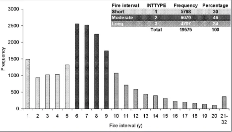
The first step was to simplify the ALLINT column to three classifications: short (≤5 yr), moderate (6 yr to 9 yr), and long (≥10 yr) fire return intervals. The number of classifications and the range they encompass can all be dic-tated by the user, though our method allows for a maximum of ten as we use single num-bers (0 to 9) for the classifications. For exam -ple, very short and very long intervals could be included. To define our short fire return inter -vals, we investigated juvenile periods of floris -tic taxa (Burrows et al. 2008), and to define our long return intervals, we investigated the time-since-fire at which fuels will carry an in -tense fire under normal (not extreme) weather conditions (Gould et al. 2007).
A B C D E F G H
1 RECNO1 YEAR FIREFREQ72 INTERVAL1 INTERVAL2 INTERVAL3 INTERVAL4 ALLINT 2 654 2002 5 12 0 0 0 12 3 654 1990 5 0 4 0 0 4 4 654 1986 5 0 0 5 0 5 5 654 1981 5 0 0 0 9 9 6 654 1972 5 0 0 0 0 0 7 653 2002 4 11 0 0 0 11 8 653 1991 4 0 7 0 0 7 9 653 1984 4 0 0 9 0 9 10 653 1975 4 0 0 0 0 0 11 652 2002 3 11 0 0 0 11 12 652 1991 3 0 19 0 0 19 13 652 1972 3 0 0 0 0 0 14 651 2002 5 8 0 0 0 8 15 651 1994 5 0 10 0 0 10 16 651 1984 5 0 0 4 0 4 17 651 1980 5 0 0 0 4 4 18 651 1976 5 0 0 0 0 0 19 650 2002 2 30 0 0 0 30 20 650 1972 2 0 0 0 0 0 D2 =
IF(((A2<A1)*AND(A2=A3)),(b2-b3),0)
All these entries are ‘0’ rather than a function. This is only needed for the first spatial group in the database.
Spatial group. All have the same value for RECNO1
The columns for INTERVAL3 and INTERVAL4 are filled with zeroes because there are only two fire intervals in this spatial group
F13 =
IF(((A11<A10)*AND(A12= A11)*AND(A13=A12)* AND(A13=A14)), (B13-B14),0)
F4 =
IF(((A2<A1)*AND(A3=A2)*AND (A4=A3)*AND(A4=A5)),(b4-b5),0)
G5 =
IF(((A2<A1)*AND(A3=A2)*AND (A4=A3)*AND(A5=A4)*AND (A5=A6)),(b5-b6),0)
H7 =
IF(D7>0,D7,IF(E7>0,E7,IF(F7>0, F7,IF(G7>0,G7,0))))
The final row in a spatial group will always return a ‘0’ under fire interval columns because the number of fire intervals is the total number of fires minus 1. For example, H10 =
IF(D10>0,D10,IF(E10>0,E10,IF (F10>0,F10,IF(G10>0,G10,0)))) E3 =
IF(((A2<A1)*AND(A3=A2) *AND(A3=A4)),(b3-b4),0)
Figure 3. Excerpt from the MS Excel file used for calculating actual fire return intervals for five polygons (spatial groups) in the dataset. We have omitted columns that are irrelevant to the computation of the fire return intervals. Boxes represent the logical test functions that have been written to compute the values for the highlighted cell. For the logical test functions in each box, the value returned in the cell is highlighted in bold (either ‘value if true’ or ‘value if false’). Where it is ‘value if false,’ the section of the logical test that is not upheld is highlighted in bold italic.
Cell value (ALLINT) =
IF(INTERVAL1>0,INTERVAL1, IF(INTERVAL2>0,INTERVAL2, IF(INTERVAL3>0,INTERVAL3, IF(INTERVAL4>0,INTERVAL4,0)))).
Juvenile period is defined as the time taken for a floristic species to reproduce following fire (Gill 1975), and the occurrence of lethal fire during the juvenile period can lead to lo -calised extinction of the species (Gill and Nicholls 1989, Burrows and Friend 1998). Therefore, Gill and Nicholls (1989) suggest that to maintain community composition, the minimum fire return interval should be based around the conservative approach of doubling the juvenile period of the slowest maturing and fire sensitive species. Based on this recom -mendation, Burrows and co-workers defined a high fire frequency (synonymous with a re -gime of short fire return intervals) as one fire at fewer than six-year intervals for the envi-ronment in which our study occurred (Burrows and Friend 1998, Burrows et al. 2008). Hence, we defined our short fire return interval as be -ing five years or less.
To define long fire return intervals, we took a risk management approach. We defined long
intervals as those of ten years or more, based on fire hazard and fuel age. In particular, sur -face fuel hazard scores, defined by Gould et al.
(2007), begin to plateau at ten years after fire in southern jarrah forest. It is the surface fuel layer that constitutes the bulk of fuel consumed and contributes most of the energy released by fire (Gould et al. 2007). Therefore, we consid -ered ten years to be a reasonable starting point for a long interval in relation to fire hazard. In addition, our data analysis was constrained by the retrospective nature of the study. In this highly managed landscape, less than one quar -ter of the total number of fire return in-tervals across space and time were ten years or greater (Figure 4).
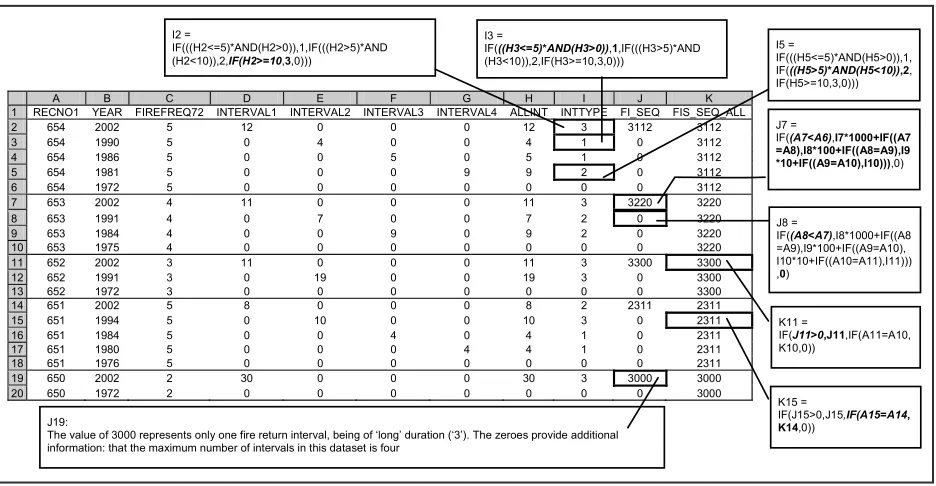
The column INTTYPE was created to con -vert the real fire return intervals under ALLINT into the following integer classifications: 1 = short (≤5 yr), 2 = moderate (6 yr to 9 yr), and 3 = long (≥10 yr), using a nested logical test function of the form:
where subscript q refers to row q in the Excel spreadsheet, and the * symbol is syntax required by MS Excel to perform the function (i.e., it is not a multiplication symbol). Figure 5 shows the outcome in the Excel file, including exam -ples of functions used to generate the integer classifications from fire return intervals.
Creating Fire Return Interval Sequences
Two columns were added to the Excel file: FI_SEQ and FI_SEQ_ALL (Figure 5). The completed fire return interval sequences were calculated in these columns from classifica -tions in the INTTYPE column using a nested logical test function. The aim of this function was to transpose the vertical classifications
that appear under INTTYPE to a horizontal se -quence of the classifications, which is a whole number made up of 1s, 2s, and 3s. This whole number indicates the temporal sequence of fire return interval classifications and is contained within a single cell and therefore available for mapping and labelling in GIS. A key part of calculating the four-digit whole number that represents the fire return interval sequence is a simple step of multiplying each value under INTTYPE by decreasing factors of 10, and adding them together. In this case, the se -quence is a four-digit number because we have a maximum of four fire return intervals in our dataset. Adjustments can be made to the cal -culations to allow for less or more intervals by decreasing or increasing the multiplication fac-tors respectively.
To calculate the fire return interval se -quence in the qth row of the FI_SEQ column, the following logical test function applies: Cell value (INTTYPEq) =
IF(((ALLINTq<=5)*AND(ALLINTq>0)),1, IF(((ALLINTq >5)*AND(ALLINTq <10)),2, IF(ALLINTq >=10,3,0))),
(3)
A B C D E F G H I J K
1 RECNO1 YEAR FIREFREQ72 INTERVAL1 INTERVAL2 INTERVAL3 INTERVAL4 ALLINT INTTYPE FI_SEQ FIS_SEQ_ALL 2 654 2002 5 12 0 0 0 12 3 3112 3112 3 654 1990 5 0 4 0 0 4 1 0 3112 4 654 1986 5 0 0 5 0 5 1 0 3112 5 654 1981 5 0 0 0 9 9 2 0 3112 6 654 1972 5 0 0 0 0 0 0 0 3112 7 653 2002 4 11 0 0 0 11 3 3220 3220 8 653 1991 4 0 7 0 0 7 2 0 3220 9 653 1984 4 0 0 9 0 9 2 0 3220 10 653 1975 4 0 0 0 0 0 0 0 3220 11 652 2002 3 11 0 0 0 11 3 3300 3300 12 652 1991 3 0 19 0 0 19 3 0 3300 13 652 1972 3 0 0 0 0 0 0 0 3300 14 651 2002 5 8 0 0 0 8 2 2311 2311 15 651 1994 5 0 10 0 0 10 3 0 2311 16 651 1984 5 0 0 4 0 4 1 0 2311 17 651 1980 5 0 0 0 4 4 1 0 2311 18 651 1976 5 0 0 0 0 0 0 0 2311 19 650 2002 2 30 0 0 0 30 3 3000 3000 20 650 1972 2 0 0 0 0 0 0 0 3000
I3 =
IF(((H3<=5)*AND(H3>0)),1,IF(((H3>5)*AND (H3<10)),2,IF(H3>=10,3,0)))
I5 =
IF(((H5<=5)*AND(H5>0)),1, IF(((H5>5)*AND(H5<10)),2, IF(H5>=10,3,0)))
J7 =
IF((A7<A6),I7*1000+IF((A7 =A8),I8*100+IF((A8=A9),I9 *10+IF((A9=A10),I10))),0)
J8 =
IF((A8<A7),I8*1000+IF((A8 =A9),I9*100+IF((A9=A10), I10*10+IF((A10=A11),I11))) ,0)
K11 =
IF(J11>0,J11,IF(A11=A10, K10,0))
I2 =
IF(((H2<=5)*AND(H2>0)),1,IF(((H2>5)*AND (H2<10)),2,IF(H2>=10,3,0)))
K15 =
IF(J15>0,J15,IF(A15=A14, K14,0))
J19:
The value of 3000 represents only one fire return interval, being of ‘long’ duration (‘3’). The zeroes provide additional information: that the maximum number of intervals in this dataset is four
where subscripts p, q, r, s, and t represent or -dered rows in the Excel spreadsheet, and * represents the multiplication function.
FI_SEQ shows the sequence of fire return interval classifications in reverse time series (i. e., most recent back to the oldest fire return in -terval; see column J in Figure 5). FI_SEQ only shows the fire return interval sequence in the first row of each spatial group (Figure 5). This is because the logical test will be false for sub-sequent cells until it reaches the first row of a new spatial group (for example, see the syntax of equation 4 and the calculations for cell J8 in Figure 5). To assign the fire return interval se -quence to all fires in a spatial group (i.e., each row), another column, FI_SEQ_ALL, was cre -ated. The reason for wanting the fire return in -terval sequence assigned to all fires in a spatial group is so that the user can obtain the fire re -turn interval sequence by selecting any of the overlapping fires within the spatial group, rath -er than only the most recent. To automate the filling of cells under FI_SEQ_ALL, another nested logical test function was written that re-lated to the values in FI_SEQ (Figure 5):
where subscripts p and q refer to subsequent rows in the Excel spreadsheet. Values in FI_ SEQ_ALL represent the sequences of fire re -turn intervals for each polygon in the dataset, and are the data used for mapping of temporal data.
Creating Fire Season Sequences
Creating fire season sequences followed a similar process as used for deriving fire return interval sequences, though we supplemented the information by producing a combined clas-sification for fire type (wildfire or prescribed burn) and fire season (Figure 2). The data for deriving fire season and type sequences were derived from two columns containing text. These columns were: 1) FIRETYPE, with val -ues of WF (indicating wildfire), PB (prescribed burn), or UN (unknown); and 2) SEASON, with values of SP (spring), AU (autumn), SU (summer), WI (winter), or UN (unknown). The wildfire entries contained information only for FIRETYPE (WF), whereas the PBs also contained information for SEASON. Thus, we made a single column called ALL-SEAS, which dropped the PB notation and contained only the following entries: WF, SP, AU, SU, WI, and UN. To populate the ALL -SEAS column, we used a logical test function of the form:
where subscript q refers to row q in the Excel spreadsheet (Figure 6). Thus, for a given row, if FIRETYPE is wildfire (WF), a WF is re -turned in the cell under ALLSEAS (the ‘value if true’). However, if that row represents a PB, then the season of that burn (given in column SEASON) is returned into the ALLSEAS col -umn (the ‘value if false’).
We then substituted a numerical classifica -tion for each of the fire types by creating the column NUMSEAS and writing a nested logi -cal test function that related back to ALLSEAS and FIRETYPE. The form of the function for NUMSEAS is shown in Figure 6 (column G), and substitutes integers for the FIRETYPE/ SEASON combinations (the classifications are shown in Table 1).
Cell value (FI_SEQq) = IF((RECNO1q<RECNO1p),
INTTYPEq*1000+IF((RECNO1q=RECNO1r), INTTYPEr*100+IF((RECNO1r=RECNO1s), INTTYPEs*10+IF((RECNO1s=RECNO1t), INTTYPEt))),0)
(4)
Cell value (FI_SEQ_ALLq) = IF(FI_SEQq>0,FI_SEQq,
IF(RECNO1q=RECNO1p,FI_SEQ_ALLp, 0))(5)
Cell value (ALLSEASq)=IF(FIRETYPEq =
Constructing sequences of fire season data followed the same procedure used for fire re -turn intervals. However, unlike fire re-turn in -tervals, which require two fires to calculate,
we were looking at data associated with every fire in the dataset. Hence, we needed to add an extra order of magnitude to the calculations to derive the sequences (see cell H7 in Figure 6). Sequences of fire season data were constructed in a column named SEAS_SEQ, and these se -quences were assigned to every fire in a spatial group under the column SEAS_SEQ_ALL (examples of logical test functions are shown in Figure 6).
Rejoining Temporal Fire Sequences with the Fire History Dataset
Using the unique identifier (RECNO2) for each record, we rejoined the calculated fire re -turn interval data (consisting of actual fire re -turn intervals in years, and the fire re-turn inter -val sequences) and the calculated fire season sequences to the FHD containing information on fires for all years (Figure 2).
A B C D E F G H I
1 RECNO1 YEAR FIREFREQ72 FIRETYPE SEASON ALLSEAS NUMSEAS SEAS_SEQ SEAS_SEQ_ALL 2 654 2002 5 WF WF 6 62651 62651 3 654 1990 5 PB AU AU 2 0 62651 4 654 1986 5 WF WF 6 0 62651 5 654 1981 5 PB UN UN 5 0 62651 6 654 1972 5 PB SP SP 1 0 62651 7 653 2002 4 WF WF 6 66220 66220 8 653 1991 4 WF WF 6 0 66220 9 653 1984 4 PB AU AU 2 0 66220 10 653 1975 4 PB AU AU 2 0 66220 11 652 2002 3 WF WF 6 66100 66100 12 652 1991 3 WF WF 6 0 66100 13 652 1972 3 PB SP SP 1 0 66100 14 651 2002 5 WF WF 6 61161 61161 15 651 1994 5 PB SP SP 1 0 61161 16 651 1984 5 PB SP SP 1 0 61161 17 651 1980 5 WF WF 6 0 61161 18 651 1976 5 PB SP SP 1 0 61161 19 650 2002 2 WF WF 6 61000 61000 20 650 1972 2 PB SP SP 1 0 61000
G2 =
IF((F2="SP"),1,IF((F2="AU"),2,IF((F2="SU"),3,IF((F2="WI"),4,IF(((F2="UN")*AND (D2="PB")),5,IF((F2="WF"),6,IF(((F2="UN")*AND(D2="UN")),7,0)))))))
H7 =
IF((A7<A6),G7*10000+IF((A7=A8),G8*1000 +IF((A8=A9),G9*100+IF((A9=A10),G10*10+ IF((A10=A11),G11)))),0)
F2 =
IF(D2="WF",D2,E2)
I19: The zeroes provide additional information: that the maximum number of fires experienced by any polygon in the database is five
H9 =
IF((A9<A8),G9*10000+IF((A9=A10),G10*10 00+IF((A10=A11),G11*100+IF((A11=A12),G 12*10+IF((A12=A13),G13)))),0)
I11 = IF(H11>0,H11,IF(A11=A10,I10,0))
I15 =IF(H15>0,H15,IF(A15=A14,I14,0))
Figure 6. Excerpt from the MS Excel file used for calculating fire season sequences for five polygons (spa -tial groups) in the dataset. We have omitted columns that are irrelevant to the computation of the fire season sequences. Boxes represent the logical test functions that have been written to compute the values for the highlighted cell. For the logical test functions in each box, the value returned in the cell is highlighted in bold (either‘value if true’ or ‘value if false’). Where it is value if true, the section of the logical test that directly produces the result is highlighted in bold italic. Where it is value if false, the section of the logical test that is not upheld is highlighted in bold italic, or where it is a nested logical test function, the part of the nested function that is upheld is highlighted in bold italic.
FIRETYPE SEASON ALLSEAS NUMSEAS
PB SP SP 1
PB AU AU 2
PB SU SU 3
PB WI WI 4
PB UN UN 5
WF WF 6
UN UN UN 7
Censored Data
By limiting our data analysis to 1972/73 onwards, there existed some fire return inter -vals that represented the time from the oldest fire back to 1972 (when a fire may or may not have occurred). Where a fire did not occur, these censored data (Polakow and Dunne 1999, Moritz et al. 2009) represent non-real fire re -turn intervals and were therefore ignored.
The dataset also contained a recent, incom-plete fire return interval (equivalent to time since the most recent fire). We have not al -lowed for this incomplete interval as the ex-perimental design for our case study described below stipulated a consistent time-since-fire for all sites. Hence, although there was a re -cent, incomplete fire return interval within each polygon, it was equal for all.
CASE STUDY:
DESIGNING A RETROSPECTIVE STUDY TO INVESTIGATE EFFECTS OF
FIRE REGIME ON bIOTA
We used the temporal sequences to investi -gate experimental design options for a study investigating contrasting fire regimes and their effects on components of the biota (Wittkuhn
et al. 2009). Our study maintained a constant
time-since-fire by restricting the study area to ~50 000 ha that burnt in either prescribed burns
of November 2002, or a wildfire of March 2003 (the 2002/03 fire-year; Figure 1). We did this to remove the time-since-fire effect on the results of the study, which can be significant for all components of the biota in southwestern Australia (Bell and Koch 1980, Burrows and Wardell-Johnson 2003, van Heurck and Abbott 2003, Robinson et al. 2008).
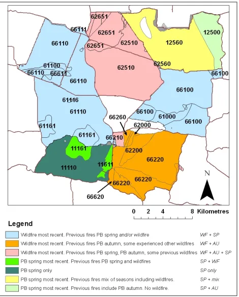
Using ArcGIS 9.0, we first investigated the sequences of fire seasons by labelling all poly -gons using values in SEAS_SEQ and visually inspecting the results (Figure 7). Using this technique, we readily identified those areas burnt most recently by wildfires and those burnt most recently by PBs. We then used the
‘Select polygons by attributes’ command in ArcGIS 9.0 to further refine historical patterns in burning histories into the following groups:
(1) wildfire most recent fire; previous fires pre -scribed in spring, some also experiencing other wildfires;
(2) wildfire most recent fire; previous fires pre -scribed in autumn, some also experiencing other wildfires;
(3) wildfire most recent fire; previous fires both spring and autumn PBs, some also ex-periencing other wildfires and PBs of un -known seasons;
(4) PB spring most recent fire; previous fires PB spring and wildfires;
(5) PB spring the only fire type;
(6) PB spring most recent fire; previous fires a mix of seasons and wildfires; and
(7) PB spring most recent fire; previous fires in -clude PB in autumn, no wildfires (Figure 7).
To investigate fire return interval sequenc -es, we were interested in the occurrence of successive short or long fire return intervals given their potential to influence species com -position (Cary and Morrison 1995). We inves -tigated the mapped fire return interval sequenc -es to identify polygons with the following pat-terns (Figure 8):
(1) consecutive short intervals (short-short = those with 11 in the sequence);
(2) consecutive long intervals (long-long = those with 33 in the sequence);
(3) mixed intervals (any combination of 1s, 2s, or 3s, but not with 11 or 33 in the se-quence), or moderate intervals (made up predominantly of 2s in the sequence).
for biological surveying (Figure 8). This area had a 30-year fire return interval prior to the most recent fire, which is significant for the re -gion (Figure 4) and would be an important in -clusion in a survey investigating the influence of long fire return intervals on the biological community.
We combined the investigation of fire sea -son sequences and fire return interval sequenc -es by creating individual shapefil-es for the short-short, long-long, mixed-moderate and 30-year interval fire interval sequences, retain -ing all the attribute information, includ-ing SEAS_SEQ. Each fire return interval group was then divided into fire season patterns by selecting polygons in ArcGIS 9.0 that related to the seven groups described above and shown in Figure 7.
Twelve contrasting fire regimes were iden -tified by combining the visual analyses of fire season and fire return interval sequences (Fig -ure 9). These regimes were based primarily on four patterns of fire return interval sequence: short-short, long-long, mixed-moderate and 30-year interval; and secondarily on seven pat-terns of fire season sequences (Table 2 and Figure 9). These factors did not occur univer -sally in combination, which would restrict the experimental design of a study investigating the complete range of fire regimes in the area.
To determine the experimental design of our case study, we gave higher priority to the fire return interval pattern over season pattern because previous work has demonstrated the importance of fire return interval sequences on biota (Cary and Morrison 1995, Watson and Wardell-Johnson 2004), and because of the fact that there were no homogenous sequences of a fire season due to the dominance of wild -fires throughout the fire history (Figure 7). Patterns in fire season sequences were more strongly aligned to the absence of a certain season rather than the predominance of a par-ticular one. The most obvious initial pattern was the type of fire experienced most recently: either wildfire or a PB in spring. For those ar -eas burnt most recently in wildfires, we noticed
further temporal patterns, particularly the oc-currence of spring or autumn PBs in the ab-sence of other seasons (Figure 7).
One drawback to undertaking a retrospec-tive study such as this is the difficulty of find -ing replicate sites that combine all the factors identified in the historical dataset. The mixed-frequency fire regime contained the widest spread of fire season patterns, though the num -ber of polygons available for site selection was few (Table 2). Both the spread of fire season patterns and number of polygons available for site selection reduced for the short-short and long-long fire return interval patterns, com -mensurate with their reduced area in relation to the mixed-frequency regime. The results suggest that it will be difficult to develop a study with suitable replicates based on past fire season sequences, but a study investigating the contrasting fire return interval sequences would provide an adequate number of replicate sites (Table 2).
DISCUSSION
We have described a technique for creating sequences of fire return interval and fire season classifications from complex spatio-temporal data to display it in a GIS. We have provided an Excel file for creating the sequences with logical test functions pre-written as supple-mentary material available from the primary author. The Excel format is useful as it is fa-miliar to many users, rather than software for spatio-temporal databases that is either still in development (Abraham and Roddick 1999), expensive to obtain, or designed for the GIS specialist. While we acknowledge the future for fire history data is in highly functional spa -tio-temporal databases (see Yuan 1997), our work fills a current gap in computational re -quirements for recognising broad patterns in spatio-temporal fire data that may be useful to fire ecologists with limited GIS knowledge.
Pattern of fire season sequence
Pattern of fire interval sequence
Short-short moderateMixed- Long-long interval30-year Total
WF+SP 3 4 3 1 11
WF+AU - 6 - - 6
WF+AU+SP 2 1 - - 3
SP+WF 1 1 - - 2
SP only - 1 - - 1
SP + mix* - - 1 - 1
SP+AU - - 1 - 1
Total 6 13 5 1 25
Table 2. Number of spatially explicit polygons for each combination of fire return interval and fire season sequence for the case study investigating contemporary fire regimes in southwestern Australia. Polygons <100 ha have been omitted. For fire season sequences: where a pattern begins with WF, this indicates the most recent fire was a wildfire; where a pattern begins with SP, this indicates the most recent fire was a pre -scribed burn in spring. Types/seasons written after the + sign indicate the other types of fires experienced historically. WF = wildfire, SP = spring prescribed burn, AU = autumn prescribed burn.
the data applies because they represent cate-gorical data. We highlighted the utility of de-veloping fire return interval and season se -quences through the investigation of experi -mental design options for a retrospective study of the effects of contrasting fire regimes on bi -ota of southwestern Australia. We see this type of data presentation as having wide application to land management authorities, as well as re-search personnel who are trying to identify patterns in their spatio-temporal data. The technique described in this paper is useful for investigating a snapshot of any form of spatio-temporal data. While we have used it for fire data, similar versions could be used for other forms of spatio-temporal data for which se-quences of events are of interest. The tech
-nique could also be used to demonstrate chang -es to individual-based or point-based data. Examples of this may be bird or animal sur-veys or water quality data where counts or measures are classified and mapped in time se -quences to demonstrate changes through time across the landscape. The main benefit of this technique, and the reason we investigated it in our study, was to provide a broad overview of the temporal patterns in data, and how they were arranged across the landscape. The ad-vantage of doing this in a GIS is that additional themes can be added such as vegetation types, geology, hydrology, or rainfall that may corre-late with spatial differences between temporal patterns.
* SP + mix has a mix of many fire types/seasonswith no discernible pattern, including prescribed burn(s) in unknown
season(s).
ACKNOWLEDGEMENTS
LITERATURE CITED
Abraham, T., and J.F. Roddick. 1999. Survey of spatio-temporal databases. GeoInformatica 3: 61-99. doi: 10.1023/A:1009800916313
Andersen, A.N. 2003. Burning issues in savanna ecology and management. Pages 1-14 in: A.N. Andersen, G.D. Cook, and R.J. Williams, editors. Fire in tropical savannas: the Kapalga ex -periment. Springer-Verlag, New York, New York, USA. doi: 10.1007/0-387-21515-8_1
Bell, D.T., and J.M. Koch. 1980. Post-fire succession in the northern jarrah forest of Western Australia. Australian Journal of Ecology 5: 9-14. doi: 10.1111/j.1442-9993.1980.tb01226.x
Boer, M.M., R.J. Sadler, R.S. Wittkuhn, L. McCaw, and P.F. Grierson. 2009. Long-term impacts of prescribed burning on regional extent and incidence of wildfires—evidence from fifty years of active fire management in SW Australian forests. Forest Ecology and Management 259: 132-142. doi: 10.1016/j.foreco.2009.10.005
Bradstock, R.A., M. Bedward, A.M. Gill, and J.S. Cohn. 2005. Which mosaic? A landscape eco -logical approach for evaluating interactions between fire regimes, habitat and animals. Wild -life Research 32: 409-423. doi: 10.1071/WR02114
Brockett, B.H., H.C. Biggs, and B.W. van Wilgen. 2001. A patch mosaic burning system for conservation areas in southern African savannas. International Journal of Wildland Fire 10: 169-183. doi: 10.1071/WF01024
Burrows, N., and I. Abbott. 2003. Fire in south-west Western Australia: synthesis of current knowledge, management implications and new research directions. Pages 437-452 in: I. Ab -bott and N. Burrows, editors. Fire in ecosystems of south-west Western Australia: impacts and management. Backhuys Publishers, Leiden, The Netherlands.
Burrows, N., and G. Wardell-Johnson. 2003. Fire and plant interactions in forested ecosystems of south-west Western Australia. Pages 225-268 in: I. Abbott and N. Burrows, editors. Fire in ecosystems of south-west Western Australia: impacts and management. Backhuys Publish-ers, Leiden, The Netherlands.
Burrows, N.D. 2008. Linking fire ecology and fire management in south-west Australian forest landscapes. Forest Ecology and Management 255: 2394-2406. doi: 10.1016/j.
foreco.2008.01.009
Burrows, N.D., and G. Friend. 1998. Biological indicators of appropriate fire regimes in south -west Australian ecosystems. Pages 413-421 in: T.L. Pruden and L.A. Brennan, editors. Fire in ecosystem management: shifting the paradigm from suppression to prescription. Tall Tim-bers Fire Ecology Conference 20th Proceedings. Tall TimTim-bers Research Station, Tallahassee, Florida, USA.
Burrows, N.D., G. Wardell-Johnson, and B. Ward. 2008. Post-fire juvenile period of plants in south-west Australia forests and implications for fire management. Journal of the Royal Soci -ety of Western Australia 91: 163-174.
Cadenasso, M.L., S.T.A. Pickett, and J.M. Grove. 2006. Dimensions of ecosystem complexity: heterogeneity, connectivity, and history. Ecological Complexity 3: 1-12. doi: 10.1016/j. ecocom.2005.07.002
Cary, G.J. 2002. Importance of a changing climate for fire regimes in Australia. Pages 26-46 in: R.A. Bradstock, J.E. Williams, and A.M. Gill, editors. Flammable Australia: the fire regimes and biodiversity of a continent. Cambridge University Press, United Kingdom.
Fulé, P.Z., W.W. Covington, and M.M. Moore. 1997. Determining reference conditions for eco -system management of southwestern ponderosa pine forests. Ecological Applications 7: 895-908. doi: 10.1890/1051-0761(1997)007[0895:DRCFEM]2.0.CO;2
Gill, A.M. 1975. Fire and the Australian flora: a review. Australian Forestry 38: 4-25.
Gill, A.M., and A.O. Nicholls. 1989. Monitoring fire-prone flora in reserves for nature conserva -tion. Pages 137-151 in: N. Burrows, L. McCaw, and G. Friend, editors. Proceedings of a na -tional workshop: fire management on nature conservation lands. Department of Conservation and Land Management Western Australia Occasional Paper 1/89.
Gould, J.S., W.L. McCaw, N.P. Cheney, P.F. Ellis, I.K. Knight, and A.L. Sullivan. 2007. Project Vesta—fire in dry eucalypt forest: fuel structure, fuel dynamics and fire behaviour. Ensis-CSIRO, Canberra, Australian Capital Territory, and the Department of Environment and Con -servation, Perth, Western Australia.
Hamilton, T., R.S. Wittkuhn, and C. Carpenter. 2009. Creation of a fire history database for southwestern Australia: giving old maps new life in a Geographic Information System. Con -servation Science Western Australia 7(2): 429-450.
Levin, S.A. 1992. The problem of pattern and scale in ecology. Ecology 73: 1943-1967. doi:
10.2307/1941447
McCaw, L., T. Hamilton, and C. Rumley. 2005. Application of fire history records to contempo -rary management issues in south-west Australian forests. Pages 555-564 in: M. Calver, H. Bigler-Cole, G. Bolton, J. Dargavel, A. Gaynor, P. Horwitz, J. Mills, and G. Wardell-Johnson, editors. A forest consciousness: proceedings of the 6th National Conference of the Australian Forest History Society. 12-17 September 2004, Augusta, Western Australia. Millpress, Rot -terdam, Netherlands.
Morgan, P., C.C. Hardy, T.W. Swetnam, M.G. Rollins, and D.G. Long. 2001. Mapping fire re -gimes across time and space: understanding coarse and fine-scale fire patterns. International Journal of Wildland Fire 10: 329-342. doi: 10.1071/WF01032
Moritz, M., T. Moody, L. Miles, M. Smith, and P. de Valpine. 2009. The fire frequency analysis branch of the pyrostatistics tree: sampling decisions and censoring in fire interval data. Envi -ronmental and Ecological Statistics 16: 271-289. doi: 10.1007/s10651-007-0088-y
Pelekis, N., B. Theodoulidis, I. Kopanakis, and Y. Theodoridis. 2005. Literature review of spa -tio-temporal database models. The Knowledge Engineering Review 19: 235-274.
Polakow, D.A., and T.T. Dunne. 1999. Modelling fire-return interval T: stochasticity and censor -ing in the two-parameter Weibull model. Ecological Modell-ing 121: 79-102. doi: 10.1016/ S0304-3800(99)00074-5
Robinson, R.M., A.E. Mellican, and R.H. Smith. 2008. Epigeous macrofungal succession in the first five years following a wildfire in karri (Eucalyptus diversicolor) regrowth forest in West -ern Australia. Austral Ecology 33: 807-820. doi: 10.1111/j.1442-9993.2008.01853.x
Van Heurck, P., and I. Abbott. 2003. Fire and terrestrial invertebrates in south-west Western Australia. Pages 291-319 in: I. Abbott and N. Burrows, editors. Fire in ecosystems of south-west Western Australia: impacts and management. Backhuys Publishers, Leiden, The Nether -lands.
Wittkuhn, R., L. McCaw, G. Phelan, J. Farr, G. Liddelow, P. van Heurck, A. Wills, R. Robinson, R. Cranfield, J. Fielder, C. Dornan, and A. Andersen. 2008. Assessing the effects of contrast -ing fire intervals on biodiversity at a landscape scale. Pages 482-493 in: Fire, environment and society: from research into practice. Proceedings of 15th annual AFAC Conference and the first International Bushfire Research Conference of the Bushfire Cooperative Research Centre, 1-3 September 2008, Adelaide, South Australia.
Wittkuhn, R.S., T. Hamilton, and L. McCaw. 2009. Fire interval sequences to aid in site selec -tion for biodiversity studies: mapping the fire regime. Proceedings of the Royal Society of Queensland (Bushfire 2006 Conference Special Edition) 115: 101-111.