www.mech-sci.net/2/197/2011/ doi:10.5194/ms-2-197-2011
©Author(s) 2011. CC Attribution 3.0 License.
Mechanical
Sciences
Open Access
Basic principles and aims of model order reduction
in compliant mechanisms
M. R¨osner and R. Lammering
Institute for Mechanics, Helmut-Schmidt-University/University of the Federal Armed Forces Hamburg, Holstenhofweg 85, 22043 Hamburg, Germany
Received: 25 February 2011 – Revised: 23 May 2011 – Accepted: 26 July 2011 – Published: 17 October 2011
Abstract. Model order reduction appears to be beneficial for the synthesis and simulation of compliant mech-anisms due to computational costs. Model order reduction is an established method in many technical fields for the approximation of large-scale linear time-invariant dynamical systems described by ordinary differential equations. Based on system theory, underlying representations of the dynamical system are introduced from which the general reduced order model is derived by projection. During the last years, numerous new pro-cedures were published and investigated appropriate to simulation, optimization and control. Singular value decomposition, condensation-based and Krylov subspace methods representing three order reduction methods are reviewed and their advantages and disadvantages are outlined in this paper. The convenience of apply-ing model order reduction in compliant mechanisms is quoted. Moreover, the requested attributes for order reduction as a future research direction meeting the characteristics of compliant mechanisms are commented.
1 Introduction
A new approach to develop a feed unit of small machine tools for small workpieces is based on the application of compliant mechanisms. Currently, non-intuitive design and optimiza-tion techniques are in progress as well as controlling, mea-suring and calibration strategies. To describe the mechanical behavior of a feed unit in an accurate way, very large and sparse finite element models arise. This leads to numerical simulations which require an unacceptable amount of time and memory space and motivates the introduction and appli-cation of model order reduction (MOR) methods. In this pa-per, MOR approaches are reviewed taking a first step towards its implemention in compliant mechanisms. To the authors’ knowledge, applications and investigations of MOR in CMs are not existent.
In the present case, the feed unit consists of two major parts: (a) the compliant mechanism (CM) is a mechanical structure consisting of flexure hinges and rigid regions, in-cluding piezo-electric actuators and (b) the measure and con-trol system supplying appropriate input signals for the me-chanical structure via the actuators. Figure 1 illustrates a prototype of a CM appropriate to novel machine tools (the
Correspondence to: M. R¨osner
actuators are not shown), as described by Wulfsberg et al. (2010), embedded in the mechatronic system.
The utilization of CMs assuring the trajectory of the tool is constituted by their performance. CMs distinguish from previous standard machine tools being potentially more ac-curate, better scalable, cleaner, low-maintenance, less noisy and cheaper in manufacturing which makes them particularly suitable for small-scale applications.
2 System theoretical background
Assuming a linear time invariant system (LTI), the perfor-mance of the compliant mechanism can be specified by a system of second order ordinary differential equations (ODE) derived from linear finite element discretization, see e.g. Koutsovasilis and Beitelschmidt (2008). This system de-scribes the reaction of the mechanical structure in answer to inputs from the control system and can be written in the time domain by means of the state space form in vectorial repre-sentation as:
Meq(t)¨ +Deq(t)˙ +Keq(t)=Beu(t),
y(t)=Ceq(t), (1)
where Me∈Rn×n mass matrix, De∈
Rn×n damping matrix,
Ke∈Rn×nstiffness matrix, Be∈
Piezo-electric Actuators
Compliant Mechanism Default
Trajectory Controller Positioning
Sensors
Figure 1.Prototype of a compliant mechanism used in a feed unit for novel machine tools as component of the mechatronic system.
output matrix selecting the y(t)∈Rmoutput vector of inter-est of the q(t)∈Rninternal state vector corresponding to the structural characteristics of the CM. Moreover, n is the order of the system, also referred to as state space dimension. In case m=p=1 and therefore Beand Ceswitch over to vec-tors as well as u(t) and y(t) to scalars, the systems is called single input – single output (SISO) otherwise multiple input – multiple output (MIMO).
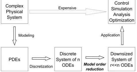
To accurately reproduce the structural behavior, in most instances, the set of ODEs stated in Eq. (1) reaches a nu-merousness of degrees of freedom (DOF), stated by n in the present case. These large scale systems entail prohibitive computational time and memory space for calculation mak-ing them impractical for simulation, optimization, analysis and control. Therefore, MOR techniques are implemented to gain a low dimensional approximation of the high order system. MOR can be arranged in the simulation process, as shown in Fig. 2.
Depending on the reduction method, different representa-tions of the system are required, which are illustrated below. Several approximation methods rely on first order systems. The transformation of Eq. (1) to a first order descriptor sys-tem is realized by applying the state vector x(t)=[qT|q˙T]T leading to the state-space dynamical system
E ˙x(t)=Ax(t)+Bu(t),
y(t)=Cx(t), (2)
where A∈Rns×ns system matrix, B∈
Rns×pinput matrix, C∈ Rm×nsoutput matrix, E∈Rns×nsdescriptor matrix and ns=2n.
Since some reduction methods are not based on the represen-tations written in Eqs. (1) and (2), respectively, but on the transfer function matrix H(s). Its derivation is described in the following.
Downsized System of r<<n ODEs Control Simulation
Analysis Optimization Complex
Physical System
PDEs
Discrete System of n
ODEs
Modeling
Discretization
Application
Model order reduction
Expensive
Figure 2.Classification of model order reduction in the simulation process of a dynamical system.
Using the Laplace transformation, the system specified in Eq. (1) is converted from time to frequency domain resulting in an algebraic system of equations given by
s2MeQ(s)+sDeQ(s)+KeQ(s)=BeU(s),
Y(s)=CeQ(s),
(3)
where s is the complex-valued scalar parameter and Q(s), U(s), Y(s) are the Laplace transformed of q(t), u(t), y(t) and provided that homogeneous initial conditions q(t=0)=q(t˙ = 0)=0 are existent.
The transfer function matrix H(s) of the system can be specified by combining the two equations in Eq. (3), as
Y(s)=Ce[s2Me+sDe+Ke]−1Be
| {z } H(s)
U(s),
(4)
alternatively for the descriptor system in Eq. (2)
H(s)=C(sE−A)−1B, (5)
where the transfer function matrix H(s) has a dimension of (m×p) in the MIMO case and, accordingly, is a scalar in the
SISO case. The transfer function H(s) describes the corre-lation between input U(s) and output Y(s), disregarding the internal states of the system.
Due to the fact that most MOR procedures are accom-plished by means of projection, the approach is explained by a system represented in Eq. (2). The objective is to approx-imate the state vector x(t)∈Rns to a low-dimensional sub-space. This is achieved by the substitution
x(t)=Vxr(t)+(t), (6)
where V∈Rns×q is the transformation matrix, xr(t)∈
Rq the
reduced state vector, (t) the residual and qns. Insert-ing the projection Eq. (6) into the linear system of ODEs in Eq. (2) results in a low-dimensional approximation
EV ˙xr(t)=AVxr(t)+BVu(t)+(t),
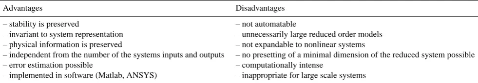
Table 1.Characteristics of condensation-based methods.
Advantages Disadvantages
– stability is preserved – not automatable
– invariant to system representation – unnecessarily large reduced order models – physical information is preserved – not expandable to nonlinear systems
– independent from the number of the systems inputs and outputs – no presetting of a minimal dimension of the reduced system possible – error estimation possible – computationally intense
– implemented in software (Matlab, ANSYS) – inappropriate for large scale systems
In general, this system is overdetermined having q unknowns but ns equations. To solve this problem and find a unique solution, Eq. (7) is pre-multiplied by a second transformation matrix W∈Rns×qsuch that WT(t)=0, the residual is equal to zero and
WTEV
| {z } Er
˙xr(t)=WTAV
|{z} Ar
xr(t)+WTB
|{z} Br
u(t),
y(t)= CV
|{z} Cr
xr(t).
(8)
The system in Eq. (8) is called general reduced order model (ROM) by projection. The number of inputs u(t)∈Rp and outputs y(t)∈Rmremains the same though the order of the system, expressed by the dimension of the reduced system matrices Er∈Rq×q, Ar∈Rq×q,Br∈Rq×p, Cr∈Rq×m and the reduced state vector xr(t)∈Rqdecreases from nsto q.
For most of the methods, the aim of model order reduc-tion is to provide the projecreduc-tion matrices W and V such that their calculation is computationally efficient as well as au-tomatable and the systems characteristics are preserved. The existence of a predefined error bound is desired in addition to the applicability in large-scale systems with an order up to a few hundred thousand. Details are specified e.g. in Eid (2009) and Rudnyi and Korvink (2006).
3 Reduction methods based on condensation
The reduction of a given system using condensation methods is the most commonly applied reduction method. Applying the time independent transformation matrices WT and V to the first equation in Eq. (1) gives the reduced system
Mr¨xr(t)+Dr˙xr(t)+Krxr(t)=Brxr(t), (9)
with Mr=WTMeV, Dr=WTDeV, Kr=WTKeV and Br= WTB
ewhere the transformation matrices have to ensure the conservation of the potential and kinetic energy of the sys-tem. The reduced damping matrix Dr may be modelled as linear combination of the mass and stiffness matrices (Rayleigh damping) with Dr=αMr+βKr.
The construction of the transformation matrix V is carried out either by static, modal or mixed condensation which are explained briefly below, see Siedl (2008), Gasch and Knothe
(1989), Bennini (2005) and Gugel (2009). In Table 1, the main advantages and disadvantages are listed for MOR using condensation-based reduction methods.
3.1 Static condensation
Static condensation is based on the partition of the systems degrees of freedom into dependent (MDOF – master degree of freedom, index m) and independent (SDOF – slave degree of freedom, index s) ones in a physical expedient way. This procedure is also the basis for sub-structure modeling and the generation of super elements. For the static case, ¨q(t) =
˙
q(t) =0, an external force vector is introduced by Beu(t) = F(t). The aforementioned partition into MDOF and SDOF applied to Eq. (1) results in
"
Kmm Kms Ksm Kss
# "
qm(t) qs(t)
#
="Fm(t)Fs(t)#. (10)
The second row in Eq. (10) provides the so called static cor-relation between the MDOF and SDOF given by
qs(t)=−K−1ssKsmqm(t)+K−1ssFs(t). (11)
One obtains the reduced system by substituting qs(t) in the first row of Eq. (10) by Eq. (11). Rearranging ensues
Kredqm(t)=Fred, (12)
where Kred =[Kmm −KmsK−1ssK−1sm] and Fred =Fm(t)− KmsK−1ssFs(t). Therewith, the transformation matrices in Eq. (8) have the following structure
V=
"
I −K−1ssKsm
# ,W=
"
I −KmsK−1ss
#
, (13)
where I is the identity matrix. The identification of Kred in this way is exact. In case of approximately reducing the mass matrix Meand damping matrix Dealso with the transforma-tion matrices in Eq. (13) from the static approach, the proce-dure is called Guyan reduction, as stated by Stelzmann et al. (2002) and Lienemann (2006).
3.2 Modal condensation
Table 2.Characteristics of Krylov subspace methods.
Advantages Disadvantages
– iterative method – no support in Matlab – easy to implement – no global error bound
– suitable for very large scale systems – order depends on number of inputs/outputs – computational efficient – result may depend on systems representation – stationary exact – no guarantee for preserving stability – robust calculation – expansion point required
on the limitation of the explorative frequency range. Resolv-ing the eigenvalue problem, neglectResolv-ing dampResolv-ing and external forces, results in the modal matrixΦassembled by the eigen-vectorsϕi
Φ=h
ϕ1, ϕ2, ···, ϕli (14)
whereΦ∈Rl×l is getting downsized by choosing a minor frequency range resulting in the reduced modal matrixΦr∈
Rl×k. Using an orthogonal projection W=V as mentioned by
Rickelt-Rolf (2009), the transformation matrices are chosen such that
W=V=Φr. (15)
3.3 Mixed condensation
Mixed condensation, known as reduction by Craig and Bampton (1968), combines static and modal reduction meth-ods. In a first step, the system in Eq. (9) is similarly re-sorted with respect to SDOF and MDOF as described before. Sec-ondly, the MDOF are blocked out by setting qm=0 resulting in an auxiliary system
Mssqs(t)¨ +Kssqs(t)=0, (16)
of which the eigenmodes ϕi are calculated subsequently. Analogue to the modal condensation, the reduced modal ma-trixΦris established by selecting certain eigenmodes as de-scribed by Siedl (2008). The SDOF is again linked to the MDOF via the static correlation and the transformation ma-trices are complemented to
W=V=
"
Φr Φs
0 I
#
(17)
withΦs=−K−1ssKsm andΦr=
h
ϕ1, ϕ2, ···, ϕkias men-tioned in Sect. 3.1 and Sect. 3.2, respectively.
4 Krylov subspace methods
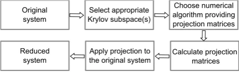
Originally, Krylov subspace methods were developed for iteratively solving large and sparse linear sys-tems of equations. Multiple methods are available,
Calculate projection matrices Choose numerical algorithm providing projection matrices Select appropriate
Krylov subspace(s)
Apply projection to the original system Original
system
Reduced system
Figure 3. Key steps of dimensional reduction using Krylov sub-spaces.
for example Generalized-Minimal-Residual-Method (GM-RES), Biconjugate-Gradient (BiCG,) Conjugate-Gradien-Square (CGS) and Transpose-Free-Quasi-Minimal-Residual (TFQMR), which can be found e.g. in Meister (2005), Kan-zow (2005), Van der Vorst (2003) and Bai (2000) to name only a few.
In case of MOR, Krylov subspaces are used to form the projection matrices V and W in Eq. (8). The general ap-proach is based on the approximation of the transfer behav-ior of the original system by means of the transfer function H(s) in the frequency domain given in Eq. (4) and Eq. (5), re-spectively. MOR using Krylov subspaces is also well-known as moment matching, meaning that a certain number of mo-ments of the reduced and the original system is equal. Hence, the moments of the transfer function and their matching in the sense of an approximation play a decisive role and are de-scribed below. Figure 3 illustrates the key steps using Krylov subspaces.
In Table 2, the main advantages and disadvantages are listed for MOR using Krylov subspaces, given in Salim-bahrami (2006) and Eid (2009).
4.1 Transfer function and its moments
Considering the transfer function in Eq. (5) for the MIMO case, rearranging results in
H(s)=−C(I−sA−1E)−1A−1B. (18)
Taking into account the Neumann series, as described by Werner (2009) and Eid (2009),
(I−sA−1E)−1= ∞
X
j=0
one obtains the following Taylor series
H(s)= ∞
X
j=0
−C(A−1E)jA−1Bsj= ∞
X
j=0
−M0jsj. (20)
This power series is called MacLaurin series, with M0
j=
C(A−1E)jA−1B called moments of the transfer function and its expansion point being s=0. Depending on the expansion point, the moments and its corresponding MOR schemes are defined as:
– Expansion point s=0 results in a MacLaurin series with its moments defined by
Msj=0=C(A−1E)jA−1B. (21)
The corresponding MOR procedure is called
Pad´e-Approximation.
– Expansion point s=skresults in a Taylor series with its moments defined by
Ms=sk
j =C((A−skE)
−1E)j(A−skE)−1B.
(22)
The corresponding MOR procedure is called Shifted
Pad´e-Approximation, Rational Interpolation or Multi-point Pad´e-Approximation.
– Expansion point s→ ∞results in a Markov series with its moments defined by
Ms→∞j =C(E−1A)jE−1B. (23)
The corresponding MOR procedure is called Partial
Re-alisation.
The users choice of the expansion point concerning its loca-tion and number in case of the Shifted Pad´e-Approximaloca-tion, which is also suitable for multiple expansion points, affects the approximating characteristics. In the context of MOR, Pad´e-Approximation matches the behavior in the low fre-quency range whereas Partial Realisation fullfils in the high frequency range and Rational Interpolation in the user spec-ified one. The usage of moment matching in sparse, large scale systems is due to the simplicity of the involved op-erations to compute these moments, namely matrix vector multiplication and matrix inversion. Details may be found in Eid (2009), Lehner and Eberhard (2006), Grimme (1997) and Salimbahrami (2006).
4.2 Krylov subspaces and moment matching
To provide the projection matrices V and W, Krylov sub-spaces are employed to match a certain number of the previ-ously defined moments. A Krylov subspace is spanned by a succession of vectors as
Kq(A,b)=span{b,Ab,A2b,...,Aq−1b}, (24)
where A∈Rn×n is a matrix, b∈
Rn is called starting vector
and b,Ab,A2b,...,Aq−1b are the generated basic vectors span-ning the q-th Krylov subspace. The first linearly independent basic vectors form the basis of this Krylov subspace. In case multiple starting vectors have to be considered, a q-th order block Krylov subspace can be rendered precisely by
Kq(A,B)=span{B,AB,A2B,...,Aq−1B}, (25)
where A∈Rn×n, B=[b1,...,bp]∈Rn×pis the starting matrix containing the p linearly independent starting vectors. If p= 1, one obtains the standard Krylov subspace in Eq. (24) with the starting vector b.
For the reduced order system in Eq. (8), the basic vec-tors of a suitable Krylov subspace can be utilized to find the projection matrices V and W. An explicit calculation of the moments to match is not neccessary. As carried out in Koutsovasilis (2009) and Salimbahrami (2006) an input block Krylov subspace Kq1(A−1E,A−1B) and output block Krylov subspace Kq2(A−TET,A−TCT) are to be used for an expansion point s=0 to match some moments in Eq. (21).
For s=sk, the input block Krylov subspace is Kq3((A− skE)−1E,(A−skE)−1B) and the output block Krylov subspace Kq4((A−skE)−TET,(A−skE)−TCT). If the colmuns of the matrix V form a basis of Kq1and Kq3, respectively, and the matrix W is chosen such that Ar=WTAV is non-singular, then the first q1m and accordingly q3m moments match. A typ-ical choice is W=V, named Galerkin (orthogonal) projec-tion, otherwise W,V Petrov-Galerkin (oblique) projection. Using only the input Krylov subspace is known as one-sided Krylov subspace method. Two-sided methods applying input and output Krylov subspaces match q1m+q2m and accordingly
q3
m+
q4
m moments.
To calculate the desired projection matrices V and W, a wide range of numerical, mostly iterative algorithms is ava-iable. The most popular ones are Arnoldi algorithm, two-sided Arnoldi algorithm and Lanczos algorithm which are not further investigated in this paper. Details and further algorithms can be found in Bechtold et al. (2007), Meis-ter (2005), Grimme (1997), Krohne (2007), Salimbahrami (2006), Antoulas et al. (2001), Eid (2009) and Bai (2002).
5 Control theory methods based on singular value
decomposition
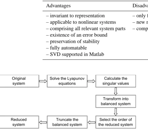
Table 3.Characteristics of SVD methods.
Advantages Disadvantages
– invariant to representation – only for small systems
– applicable to nonlinear systems – new methods may have convergence troubles – comprising all relevant system parts – computationally expensive (Lyapunov equations) – existence of an error bound
– preservation of stability – fully automatable – SVD supported in Matlab
Transform into balanced system Solve the Lyapunov
equations
Calculate the singular values Original
system
Select the order of the reduced system Truncate the
balanced system Reduced
system
Figure 4.Key steps of dimensional reduction using singular value decomposition (SVD).
5.1 Controllability and observability of a system Considering the system in Eq. (2) represented by
˙x(t)=Ax(t)ˆ +Bu(t)ˆ ,
y(t)=Cx(t), (26)
the two important control theory quantaties controllabilityP and observability Qcan be introduced, as done by Liene-mann (2006), via the Gramians
P=
Z ∞
0
eAtˆ B ˆˆBTeAˆTtdt (27)
and
Q=
Z ∞
0
eAˆTtCTCeAtˆ dt. (28)
The concept of controllability examines how the states x(t) of a system are linked to its inputs u(t) whereas observabil-ity deals with the connection between the states x(t) and its outputs y(t), as delineated by Eid (2009).
Under certain conditions, described e.g. by Bechtold et al. (2007) and Koutsovasilis (2009), the Gramians can be found by solving the two system related Lyapunov equations given by
ˆ
AP+PAˆT+B ˆˆBT=0,
ˆ
ATQ+QAˆ+CTC=0. (29)
5.2 The singular value decomposition
As known from linear algebra and described by Gugel (2009) and Hackbusch (2009), any matrix A∈Rm×ncan be decom-posed into the product of three matrices, more precisely an orthogonal matrix U, a diagonal matrixΣand the transpose of an orthogonal matrix V such that
A=UΣVT= k
X
i=1
σiuivTi (30)
where the matrix
ˆ
Σ=
σ1 ··· 0
..
. ... ...
0 ··· σk
,Σ="Σˆ 0
0 0
#
∈Rm×n (31)
comprises the singular valuesσi =
pλ
i(ATA) ≥σi+1 ≥0 on
its diagonal in descending order with rank(A) =k and k =
min{m,n}. The left singular vectors U=[u1u2...um]∈Rm×m
are the orthonormal vectors of A AT, the right singular vec-tors V=[v1v2...vn]∈Rn×n are the orthonormal vectors of ATA. The term in Eq. (30) is called a singular value decom-position (SVD) of A and provides a basis for finding a lower ranked matrix Arwhich best approximates A such that
Ar= r
X
i=1
σiuivTi. (32)
The task is to find an optimal approximation in a certain sys-tem norm, eg. the spectral norm (H2-norm), as specified by Antoulas and Sorensen (2001), Hackbusch (2009) and Dah-men and Reusken (2008), via the Schmidt-Mirsky theorem which results in the minimisation of the approximation error such that
min rank(Ar)≤rank(A)
kA−ArkH2=σk+1(A). (33)
5.3 Balanced truncation approximation
In case of a stable system, balanced truncation approxima-tion (BTA) assumes that the system is balanced first and af-terwards truncated. Based on the system representation given in Eq. (26), the balanced partition of the system matrices and state vector can be quoted as
"
˙x1(t) ˙x2(t)
#
="A11ˆˆ A12ˆ
A21 Aˆ22
# "
x1(t) x2(t)
# +"B1ˆˆ
B2
#
u(t)
y(t)=hC1ˆ C2ˆ i
"
x1(t) x2(t)
# (34)
with ˆA11∈Rr×r, ˆB1∈Rr×m and ˆC1∈Rp×r. At all times, a balancing transformation is feasible for minimal order sys-tems. The McMillan degree of the system is specified as the order of any minimal state-space realization of the transfer-function matrix, as stated by Sasane (2002) and Baur and Benner (2008).
The singular values are the eigenvalues of the observability Pand controllabilityQGramians:σi=
pλ
i(PQ) which are called Hankel singular values (HSV) ofΣ, e.g. described by Gugercin and Antoulas (2004) and Antoulas and Sorensen (2001). The Gramians are equal and diagonal. The bal-anced truncation approximation is predicted on transform-ing the state-space-system into a balanced realization. Those state variables that are least observable and controllable, and therefore related to the smallest Hankel singular values, are truncated with respect to the error bound between original and reduced transfer function
kH(s)−H(s)rkH∞≤2
m
X
r+1
σi. (35)
The ROM obtained by BTA is related to
˙x1(t)=A11ˆ x1(t)+B1u(t)ˆ ,
y(t)=Cˆ1x1(t).
(36)
as mentioned by Obinata and Anderson (2000). BTA in-volves an approximation error in the low-frequency region as mentioned by Bechtold et al. (2007), Obinata and Ander-son (2000) and Baur and Benner (2008). For details and as-pects in numerical calculation see e.g. Benner and Quintana-ort’i (2004), Bechtold et al. (2007), Koutsovasilis (2009), Antoulas (2005) and Gugercin and Antoulas (2004).
5.4 Singular perturbation approximation
The singular perturbation approximation (SPA) is closely re-lated to the balanced truncation approximation and ensures zero error at zero frequency and is applicable to nonlinear systems. Refering to the expression in Eq. (34) and as ex-plained by Liu and Anderson (1989) and Antoulas et al. (2001) the reduced system is identified by
˙xr(t)=Ax(t)˜ +Bu(t)˜ ,
yr(t)=Cx(t)˜ , (37)
with the reduced system matrices ˜A=Aˆ11−Aˆ12Aˆ−122Aˆ21, ˜B= ˆ
B1−A12ˆ Aˆ−122B2ˆ and ˜C=C1ˆ −C2ˆ Aˆ−122A21. In contrast to BTA,ˆ SPA has an approximation error at high frequencies, but it matches at low frequencies, see Obinata and Anderson (2000).
5.5 Hankel norm approximation
The Hankel norm approximation (HNA) employs the so-called Hankel norm which is defined as the maximal Hankel singular value of the system given in Eq. (26):
kH(s)kH=pλmax(PQ)=σmax. (38)
The aim is to minimize the approximation error between the original system transfer function H(s) and the reduced one Hr(s) with order r via the Hankel norm
kH(s)−Hr(s)kH2=σr+1(H(s))≤ kH(s)−H˜r(s)kH, (39)
as stated by Glover (1984), Green and Limebeer (1995), Bechtold et al. (2007), Benner et al. (2004), Antoulas (2005) and Antoulas and Sorensen (2001) where also the computa-tion of the optimal Hankel norm approximacomputa-tion is performed. In Eq. (39) ˜Hr(s) denotes all transfer functions of McMillan degree less than or equal to r.
6 Conclusion: benefits and aims for model order reduction in compliant mechanisms
In this work, system theoretical basics are reviewed which constitute the origin for model order reduction (MOR). Three different procedures, namely modal reduction, Krylov sub-spaces and singular value decomposition (SVD) based meth-ods, are described with their associated characteristics.
The application of MOR can be motivated by challenges arising in the numerical characterisation of compliant mech-anisms (CM) which can be traced back to the numerousness of ODEs required to specify their behavior in an accurate way. In most cases, large finite element models arise to cap-ture a detailed representation of the geometrical domain and the dynamical performance of the CM. This circumstance is unfeasible, particularly with regard to further investigations such as simulation, optimization and control. For this reason, MOR in CMs seems to be a purposeful approach to generate efficient models and would benefit the design and develop-ment as well as analysis process of CMs.
system implying a global error bound, the procedure should preserve the passivity as well as stability, has to be automat-able, stable and computational efficient also for high order systems.
In future work, different MOR schemes applied to CM will be investigated and reasonable combinations among them will be analysed to benefit from their advantages. Further-more, a specific adjustment and upgrading is desired. Out of this, the aim is to provide a reduction procedure meeting the special circumstances of CMs.
Acknowledgements. This work is supported by the German Research Foundation (DFG) as part of the research project “SPP 1476 – Small machine tools for small workpieces” which is gratefully acknowledged.
Edited by: J. A. Gallego S´anchez Reviewed by: two anonymous referees
References
Antoulas, A.: Approximation of large-scale dynamical systems, So-ciety for Industrial Mathematics, 2005.
Antoulas, A. and Sorensen, D.: Approximation of large-scale dy-namical systems: An Overview, Int. J. Appl. Math. Comput. Sci, 11, 1093–1121, 2001.
Antoulas, A., Sorensen, D., and Gugercin, S.: A survey of model reduction methods for large-scale systems, in: Structured matri-ces in mathematics, computer science, and engineering: proceed-ings of an AMS-IMS-SIAM joint summer research conference, Vol. 280, p. 193, 2001.
Bai, Z.: Templates for the solution of algebraic eigenvalue prob-lems, Society for Industrial Mathematics, 2000.
Bai, Z.: Krylov subspace techniques for reduced-order modeling of large-scale dynamical systems, Appl. Numer. Math., 43, 9–44, 2002.
Baur, U. and Benner, P.: Gramian-Based Model Reduction for Data-Sparse Systems, SIAM J. Sci. Comput., 31, 776–798, 2008. Bechtold, T., Rudnyi, E., and Korvink, J.: Fast simulation
of electro-thermal MEMS: efficient dynamic compact models, Springer Verlag, 2007.
Benner, P. and Quintana-ort’i, E. S.: G.: Parallel model reduction of large-scale linear descriptor systems via Balanced Truncation, in: LECT NOTES COMPUT SC, Proc. 6th Intl. Meeting VEC-PAR04, 28–30 June 2004, 65–78, 2004.
Benner, P., Quintana-Orti, E., and Quintana-Orti, G.: Computing optimal Hankel norm approximations of large-scale systems, in: Decision and Control, 2004, CDC. 43rd IEEE Conference on, Vol. 3, 3078–3083, 2004.
Bennini, F.: Ordnungsreduktion von elektrostatisch-mechanischen Finite Elemente Modellen f¨ur die Mikrosystemtechnik, Ph.D. thesis, Universit¨atsbibliothek der Technischen Universit¨at, 2005. Craig, R. and Bampton, M.: Coupling of substructures for dynamic
analysis, AIAA journal, 6, 1313–1319, 1968.
Dahmen, W. and Reusken, A.: Numerik f¨ur Ingenieure und Natur-wissenschaftler, Springer, 2008.
Eid, R.: Time Domain Model Reduction by Moment Matching, Ph.D. thesis, TU M¨unchen, 2009.
Gasch, R. and Knothe, K.: Strukturdynamik, Bd. 2, Springer, New York, NY, USA, 1989.
Glover, K.: All optimal Hankel-norm approximations of linear mul-tivariable systems and their L-error bounds, Int. J. Control., 39, 1115–1193, 1984.
Green, M. and Limebeer, D.: Linear robust control, Prentice Hall, 1995.
Grimme, E.: Krylov projection methods for model reduction, Ph.D. thesis, Citeseer, 1997.
Gugel, D.: Ordnungsreduktion in der Mikrosystemtechnik, Ph.D. thesis, Universit¨atsbibliothek der TU Chemnitz, 2009.
Gugercin, S. and Antoulas, A.: A survey of model reduction by balanced truncation and some new results, Int. J. Control., 77, 748–766, 2004.
Hackbusch, W.: Hierarchische Matrizen, Springer-Verlag Berlin Heidelberg, 2009.
Kanzow, C.: Numerik linearer Gleichungssysteme: direkte und it-erative Verfahren, Springer, 2005.
Koutsovasilis, P.: Model Order Reduction in Structural Mechanics Coupling the Rigid and Elastic Multi Body Dynamics, Ph.D. the-sis, TU Dresden, 2009.
Koutsovasilis, P. and Beitelschmidt, M.: Comparison of model reduction techniques for large mechanical systems, Multibody Syst. Dyn., 20, 111–128, 2008.
Krohne, K.: Order reduction of finite-volume models and its ap-plication to microwave device optimization, Ph.D. thesis, Swiss Federal Institue of Technology Zurich, 2007.
Lehner, M. and Eberhard, P.: Model Reduction in Flexible Multi-body Systems, At.-Autom., 54, 170–177, 2006.
Lienemann, J.: Complexity reduction techniques for advanced MEMS actuators simulation, Ph.D. thesis, Universit¨atsbibliothek Freiburg, 2006.
Liu, Y. and Anderson, B.: Singular perturbation approximation of balanced systems, Int. J. Control., 50, 1379–1405, 1989. Meister, A.: Numerik linearer Gleichungssysteme: eine Einf¨uhrung
in moderne Verfahren, Vieweg+Teubner Verlag, 2005. Obinata, G. and Anderson, B.: Model reduction for control system
design, Springer Verlag, 2000.
Rickelt-Rolf, C.: Modellreduktion und Substrukturtechnik zur effizienten Simulation dynamischer, teilgesch¨adigter Systeme, Ph.D. thesis, TU Braunschweig, 2009.
Rudnyi, E. and Korvink, J.: Model order reduction for large scale engineering models developed in ANSYS, in: Lect. Notes Com-put. Sc., 349–356, Springer, 2006.
Salimbahrami, B.: Structure preserving order reduction of large scale second order models, Ph.D. thesis, TU M¨unchen, 2006. Sasane, A.: Hankel norm approximation for infinite-dimensional
systems, Springer, 2002.
Siedl, D.: Simulation des dynamischen Verhaltens von Werkzeug-maschinen w¨ahrend Verfahrbewegungen, Herbert Utz Verlag, 2008.
Stelzmann, U., Groth, C., and M¨uller, G.: FEM f¨ur Praktiker-Band 2: Strukturdynamik, Expert Verlag, 2002.
Van der Vorst, H.: Iterative Krylov methods for large linear systems, Cambridge University Press, 2003.
Werner, D.: Funktionalanalysis, Springer, 2009.