Efficient and accurate document image classification algorithms for low-end copy pipelines

R E S E A R C H

Open Access

Efficient and accurate document image

classification algorithms for low-end copy

pipelines

Wen-Hsiung Huang, Yung-Yao Chen, Pei-Yu Lin, Che-Hao Hsu and Kai-Lung Hua

Abstract

The copy mode selection, such as the text mode and photo mode, of a digital copy machine can provide suitable process and enhancement for the scanned image. To classify the scanned image without expensive hardware and reduce the running time, in this article, we designed an efficient automatic method for classifying a document image using a probabilistic decision strategy. The proposed algorithm is tailored to inexpensive hardware and significantly reduces both the running time and memory requirements compared to the existing algorithms, while substantially improving the classification accuracy. In addition, we incorporate a new classification module to help avoid moiré patterns by identifying periodic halftone noise.

Keywords: Document classification, Periodic halftone noise, Digital copier, Copy mode selector

1 Introduction

A digital copier is a very common piece of home or office equipment. Users typically just push the copy button to make a copy. Most of them are not aware of the fact that copy machines usually have various copy modes associ-ated with different rendering techniques. For example, while the text mode would enhance the edge detail, the photo mode would improve the appearance of very pale colors and smooth the scanned document for noise reduc-tion. Even if the user is aware of different copy modes, it is still cumbersome to select the appropriate copy mode page by page for multi-page documents. Hence, it is essen-tial to develop an automatic page classifier.

The low-complexity method proposed in this paper enables automatic tagging of document images in a low-end copier or all-in-one, by classifying an input original into all possible combinations of mono/color, text/mix/picture/photo, and periodic/stochastic. Note that classifying a document as a photo automatically implies stochastic halftone, hence there is no color-photo-periodic or mono-photo-color-photo-periodic class. Mono mode is a configuration optimized for monochrome originals while

*Correspondence: [email protected]

Department of Computer Science and Information Engineering, No.43, Sec. 4, Keelung Road, 106 Taipei, Taiwan

color mode is optimized for color originals. Text mode is optimized for text, line arts, simple graphics, handwritten text, and faxes; picture mode is for high dynamic range halftoned originals; photo mode is for continuous tone natural scenes; mix mode is for originals containing both text and picture content; periodic mode is for periodic halftoned printed documents, and stochastic mode is for documents printed by other methods.

Misclassifying an original from one class as any of the other classes is an error; however, not all misclassification errors are equally costly. We define two cases of misclassi-fication asbenignerror: Misclassifying mono originals as color, and misclassifying text or picture or photo originals as mix. All the other misclassification cases are considered harmfulerrors.

There is a substantial amount of literature related both to the problem of overall segmentation and classifica-tion of document images, and to the specific classificaclassifica-tion tasks considered in this paper. The literature [1, 2] is not applicable to our task due to the stringent complexity restrictions imposed by the low-end machines. Moreover, the document classification algorithms of [3–7] access the entire image all at once and visit each pixel multi-ple times—something that is impossible in the low-end machines.

A number of articles [8–10] discussed the related train-ing classifiers. The literature [9] presented the traintrain-ing classifiers using multilayer neural networks to reduce the error in a supervised learning situation. Neural Network techniques can build powerful classifiers with regulariza-tion, complexity adjustment and model adjusting. The parameters (weights) in neural network significantly influ-ence the training results. The training analysis in [9, 10] normally is a costly and time-consuming process. The article [11] using multiple instance learning (MIL) to reduce the training instances for handwritten and printed documents classifications. From the results, their scheme can achieve the similar detection accuracy as SVM for the two document image classifications. Nevertheless, the training time and testing time of MIL are still higher than support vector machine (SVM).

The scheme [12] utilizes SVM classifiers with Huffman tree architecture to classify massive documents. The SVM multiple classifiers can be constructed based on Huffman tree with the paragraph and local pixel feature of the input document images. Their scheme can distinguish the texture, character and color from the document images. However, the schemes [11, 12] are complexity and infea-sible of distinguishing different modes, such as text, pic-ture, photo, mix, and periodic, for the common scanned image. The article [13] proposed an incremental learning approach for document image with zone classification. The scheme segments the document image into physical zones according to a zone-model with incremental learn-ing. The scheme provides five classes (handwritten, tables, stamps, signatures, and logos) with 1117 zones. However, the five classes are unsuitable for applied in the digital copier. To classify biomedical document images, the article [14] extends image classification with scale invariant feature transform (SIFT) by adding color features with bags-of-colors (BoC). In [15, 16], the articles designed a document image classification using convolutional neural network (CNN) that shares weights among neurons among a layer. The schemes aim to distinguish the content of the input document image, such as the ad, email, news and report. The manner [17] can achieve higher accuracy than [15] by utilizing speeded up robust features (SURF). Conse-quently, to design an efficient copy mode selection for low-end digital copier, the complexity, time consuming and accuracy should be the major concerns.

In our previous work [1], we demonstrated that our low-complexity image classification algorithms perform with 29 to 99 % accuracy on a large dataset, where misclassifi-cations tend toward benign. Our present work improves upon [1] in two important respects:

(1) Developing new feature extraction and classification methods which result in both lower complexity and higher accuracy than the algorithm of [1]. Specifically:

• In Section 2, we propose a novel classification algorithm. We demonstrate in Section 4 that it improves the classification rate by up to 22 % points as compared to the classifier of [1], when both use the same set of low-complexity features developed in Section 3.

• In Section 3, we develop a set of features all of which, unlike the features in [1], avoid vertical filtering operations (i.e., computations that involve more than one line of data at a time) and result in 23 and 50 % reductions of the running time and memory requirements, respectively.

(2) In Section 3.5, we incorporate a periodic halftone classification module developed in [18] which can be added both to the classifier of [1] and to the classifier proposed here, in order to help avoid moiré patterns. Experimental studies in [18] and in Section 4 show that our periodic halftone detector has a97 %correct classification rate.

2 Algorithm overview and hybrid hard/soft-decision algorithm

We work with a specific copy pipeline equipped with different copy modes which are all possible combina-tions of mono/color, text/mix/picture/photo, and peri-odic/stochastic. Our goal is to classify the scanned image of the original into fourteen distinct classes. These classes are listed in the first column of Table 1, where p and s indicate periodic and stochastic, respectively. Note that classes mono-photo-p and color-photo-p are absent, since classifying a document as a photo automatically means stochastic halftone.

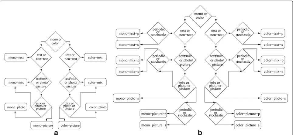
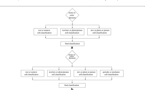
In [1], we developed an algorithm for classifying a document as combinations of mono/color and text/mix/ photo/picture. That algorithm works by sequentially applying four simple classifiers to a document: first, a classifier to distinguish color from neutral documents; second, a classifier to distinguish text from non-text doc-uments; another classifier to distinguish mix documents from photos/pictures; and a fourth classifier to decide between photos, pictures, and the mix class, as shown in Fig. 1a.

Each classifier i uses a feature vector xi consisting of one or two simple features extracted from the docu-ment image, and makes its decision based on the decision boundaries shown in Fig. 2a–d. The decision bound-aries, as well as certain parameters of the feature vectors, are estimated from training data. An additional classifier developed in [18] is depicted in Fig. 2e. It can be added to the classifier [1], as shown in Fig. 1b.

Table 1The fourteen distinct classes

Mono Color

Text Mix Pic Photo Text Mix Pic Photo

p mono-text-p mono-mix-p mono-pic-p – color-text-p color-mix-p color-pic-p –

s mono-text-s mono-mix-s mono-pic-s mono-photo-s color-text-s color-mix-s color-pic-p color-photo-s

misclassified as text by the second classifier will not be processed by the remaining classifiers. We propose to address this disadvantage by developing a hybrid hard/soft-decision algorithm where each classification node is visited, but most decisions are not made until all nodes have been traversed. Specifically, our new algorithm still starts by performing a hard decision for the neu-tral/color classifier, in order to avoid any misclassifications of color documents as mono. We retain the remaining classification nodes; however, we use them for estimat-ing class likelihoods instead of for producestimat-ing individual classification decisions. In other words, instead of pro-ducing a hard classification decision, each classifier now produces a likelihood for each class. These likelihoods are then combined to produce the final classification. This strategy produces some complexity overhead because now every image goes through every classification node. This is in contrast to the hard classification strategy of Fig. 1a where, for example, correctly classified text documents do not go through the last two classification nodes. The overhead, however, is small. The average running time per test image is approximately 0.268 s1 on an Intel(R) Core(TM) i7-4770 3.40 GHz desktop computer for our proposed soft classification algorithm. The average run-ning time for text documents in our test set for the hard

classifier is approximately 0.212 s. The average running time for mix documents for the hard classifier is approx-imately 0.259 s. For correctly classified photo and picture documents, all classification nodes of the hard classifier must be visited, and therefore the average running time for such documents is the same as for the soft classifier.

Figure 3a shows the structure of our new classifier using the classes from [1]; Fig. 3b shows the modified structure which incorporates the additional halftone classification node developed in Section 3.5.

2.1 Soft classification algorithm

As shown in Fig. 3, a hard mono-or-color decision is made at the beginning of our new classification strategy. We call the four soft classification nodes shown at the second level of Fig. 3b nodes 1, 2, 3, and 4, left to right, and let

xi be the feature vector computed at thei-th node. (The computation of feature vectors is described in the next section.)

We letX = (x1,x2,· · ·,xn) be the overall feature vec-tor obtained from all n soft classification nodes: n = 3 for Fig. 3a and n = 4 for Fig. 3b. Let cj, j = 1,· · ·,M, be the M document classes for the overall classifier, i.e., M = 8 for Fig. 3a and M = 14 for Fig. 3b. Our proposed algorithm estimates the likelihood

Fig. 2Decision boundaries for classification nodes. (a), (b), (c), (d), (e) show the decision boundaries for “mono vs color,” “text vs nontext,” “text/mix vs photo/picture,” “mix vs photo vs picture,” and “periodic vs stochastic” classification node, respectively

P(X|cj)of each classcj and classifies the document into the class that has the highest estimated likelihood. We assume conditional independence of the feature vectors computed at all nodes, given each class. Hence, each class likelihood factorizes over thenclassification nodes as follows:

P(X|cj)=

i

P(xi|cj). (1)

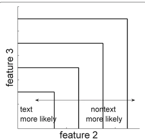
The class likelihood at each node i, P(xi|cj), is esti-mated using a five-bin histogram. The histogram bins are produced for every classifier by using four shifts of the decision boundary in Fig. 2. This is illustrated in Fig. 4 for the the text-vs-nontext classifier. In this case, the his-togram bin containing the origin represents documents that are very probable to be text documents. Going from the innermost bin to the outermost bin, the probability of text diminishes, and the probability of nontext increases.

Fig. 4Decision boundaries for the soft text-vs-nontext classifier

The innermost bin boundary is chosen to minimize the following number: (number of training text documents inside the innermost bin) - 10·(number of training nontext documents inside the innermost bin). This is illustrated in Fig. 5. The first term in this objective function reflects the fact that we would like the innermost bin to characterize text documents. The second term reflects the fact that we are willing to tolerate a relatively small number of outlier nontext documents inside the innermost bin.

Fig. 5Scatter plot of two features used in the text-vs-nontext classification for the color originals in the training suite.Blue O’s represent text documents, andred X’srepresent nontext documents

Similarly, the outermost bin boundary is chosen to min-imize the following number: (number of training nontext documents in the outermost bin) - 10·(number of train-ing text documents in the outermost bin). To obtain the remaining three bins, the distance between the inner-most and outerinner-most bin boundaries is then partitioned into three equal parts along each feature axis. The likeli-hoodP(x1|cj)of each classcjfor any feature vectorx1at the text-vs-nontext node is estimated as the value of the histogram bin whichx1belongs to. Similar histogram con-struction and likelihood estimation procedures are used for the other three soft classification nodes.

To classify a document, we employ a modified maxi-mum likelihood decision rule, constructed so as to bias the decision towards the safe “mix” classification. Given a document to classify, we extract the features, perform the mono-vs-color classification, and estimate the class likelihoods P(xi|cj) at the four soft classification nodes i=1, 2, 3, 4. We then combine these estimates via Eq. (1) to estimate the overall class likelihoodsP(X|cj). We clas-sify the document as classj∗if both following conditions hold:

ˆ

P(X|cj∗) > Pˆ(X|cj)for allj=j∗, (2)

ˆ

P(X|cj∗)

M

j=1Pˆ(X|cj)

> T, (3)

where T is a threshold parameter. In our experiments, T =0.85.2The first equation corresponds to the standard maximum likelihood classification. The second equation ensures that if there is no clear winner among the differ-ent classes, we do not declare a winner. Instead, if Eq. (3) does not hold, we default to the safe mix class. In this case for the classifier in Fig. 3b, if the maximum likelihood class is one of the periodic halftone modes, we classify the document as mix-p; otherwise, we classify it as mix-s.

3 Feature extraction

In this section, we describe all the features used in the four classifier nodes. These nodes use seven features: the mono-vs-color, photo-vs-mix-vs-picture, and periodic-vs-stochastic nodes use one feature each, and the text-vs-nontext and picture/photo-vs-mix/text nodes use two features each. Of these seven features, three are new to this work, three are taken from [1], and one is taken from [18]. We work with the same NIQ color space as [1].

3.1 Text vs. nontext classifier

• N(p1),N(p2),N(p3)are monotonically increasing or

monotonically decreasing,

• |N(p1)−N(p3)|>T1,

• |N(p0)−N(p1)|<T2and|N(p3)−N(p4)|<T2, whereN(pi)represents the luminance intensity ofpi, and T1andT2 are predefined thresholds. An image block is called a nontext block if there are no text edges in it. To compute the luminance variability score, a test image is partitioned into 8×8 blocks and the mean of each non-text block is calculated. We build a 256-bin histogram of nontext block means over the test image. Luminance vari-ability score is then defined as the number of bins whose values are greater than a predefined thresholdη.

The definition of the luminance variability score is similar to the corresponding feature in [1]; importantly, however, it avoids any vertical computations which is sig-nificant for low-complexity hardware implementations.

The second feature, histogram flatness score, is identical to [1], and uses the fact that the histogram for a typical text region has peaks that are more narrow and tall than the peaks in a typical picture or photo histogram. To compute this feature, we partition an image into 8×64 blocks and calculate a 64-bin luminance histogram for each block. Thek-span of a histogram is defined as the largest num-ber of consecutive bins in the histogram whose values exceedk. Thek-span of an image is then defined as the maximum value over all blocks. For each image, we form a n-dimensional feature vector consisting of n different k-spans, forn different values ofk. We usen= 10 and k = 15, 30,. . ., 150 as suggested by [1]. Given a fea-ture vectorx, the histogram flatness score is defined as

(mnontext−mtext)T_F−1x, wheremˆnontextandmˆtextare the estimated mean vector for the two classes; andˆF is the estimated common covariance matrix.

3.2 Text/mix vs. picture/photo classifier

There are two main differences between text/mix and pic-ture/photo documents: (1) pictures and photos contain no text; (2) pictures and photos contain natural scenes. These two properties are exploited by the two features, the text edge score and the unnaturalness score, that we designed for distinguishing text/mix documents from picture/photo documents.

To describe the text edge score, we first define ahalftone noise tripletas three consecutive pixelsp0,p1, andp2, in horizontal direction, satisfying the following conditions:

• [N(p0)−N(p1)]×[N(p1)−N(p2)]<0,

• |N(p0)−N(p1)|>T3and|N(p1)−N(p2)|>T3, where T3 is a predefined threshold. An image is parti-tioned into 64×64 blocks. For each block, we count the number of text edges (defined in the previous subsection)

and the number of halftone noise triplets. Since halftone noise generally causes false text edge detection, we define text edge score of a block as the number of text edges minus the number of halftone noise triplets. The text edge score for an image is then defined as the maximum text edge score among all blocks.

The second feature, unnaturalness score, of this classi-fier is identical to [1]. To compute it, we reuse the 256-bin histogram of 8×8 nontext block means over the image defined in Subsection 3.1. We calculate the number of nonzero bins for the histogram; furthermore, we calcu-late the k-spans for three different k: M/8, M/4, M/2, where Mis the maximum of the histogram over its 230 bins. These values form a feature vector. Given a feature vector y, we define the unnaturalness score as follows: U = (mˆtext/mix − ˆmpic/photo)Tˆ−1U y, where mˆpic/photo andmˆtext/mixare the estimated mean vectors for the two classes, and ˆU is the estimated common covariance matrix.

3.3 Picture vs. photo classifier

A picture is a halftone image; on the other hand, a photo is a continuous-tone image. We observe that smooth regions near midtone are most affected by the halftone noise. Therefore, we use these regions to distinguish between a picture and a photo.

The feature used for picture-vs-photo classifier in our algorithm is obtained from the one in [1] by removing all vertical computations. We partition an image into 8×8 blocks and measure each blockb’s noise level in the lumi-nance channel. We define a blockb’s roughnessγN(b)as follows:

γN(b)= (i,j)

|N(i)−N(j)| if| ¯N(b)−128|< φ,

∞ otherwise.

(4)

Where the summation is over all possible pairs(i,j)of horizontal neighboring pixels inside the blockb,N¯(b)is the average luminance intensity of all pixels inside the blockb, andφis a predefined threshold. The roughness of the imageγimageis defined as the minimumγ (b)over all its blocks.

3.4 Neutral vs. color classifier

We use the feature for the neutral-vs-color classifier from [1]. We define the colorfulness, C(p), of a pixel p as follows:

than a predetermined threshold; otherwise it is classified as neutral.

3.5 Periodic halftone classifier

We partition the image into 32 × 32 blocks. For each 32×32 block, we examine every inner pixel, pinner, of the block. We compare the luminance ofpinner,N(pinner), with luminance values of its four neighbor pixels:N(pleft), N(pright), N(ptop), andN(pbottom). IfN(pinner) is smaller than any three of the four luminance values from its neigh-bors, we replaceN(pinner)with zero. On the other hand, ifN(pinner)is larger than any three of the four luminance values from its neighbors, we replaceN(pinner)with 255. We let beh(x,y) denote the halftone-enhanced result of processing a blockb with this procedure where(x,y) is the block coordinate. In addition, we letB_eh(u,v)be the discrete Fourier transform (DFT) ofbeh(x,y):

Beh(u,v)= 1 MN

M−1

x=0 N−1

y=0

beh(x,y)e−j2π(ux/M+vy/N), (6)

whereM=N=32 in our case.

We define regionRof the support of|Beh(u,v)|as the union of the following two areas:

• Upper-left:u=(0, 1,. . ., 10)andv=(0, 1,. . ., 10),

• Upper-right:u=(21, 22,. . ., 31)and

v=(0, 1,. . ., 10).

We let NR denote the number of points in the region R. Note that the the regionRexcludes the low frequency components region which generally has large coefficients. In our experiments,NR=11×11×2=242. We define BmeanandBmaxas the average and maximum of|Beh(u,v)| over regionR.

We create a global histogram withNRbins, one bin for every location(u,v)in regionR. The valuehist(u,v)is the number of large maxima of|B_eh(u,v)|at frequency(u,v) over the 32×32 image blocks. The precise definition of hist(u,v)is given in the pseudocode of Fig. 6.

The feature value of the periodic halftone detector is defined as the maximum value over all the bins of the histogram.

Fig. 6Pseudocode for building the histogram of large maxima of|Beh|

4 Experimental results

In terms of memory and time complexity, our approach outperforms [1]. While the text edge and roughness fea-tures in [1] require having two strips of data in memory, there is only one strip needed in our algorithm—a 50 % reduction in memory requirements. In addition, since we remove the vertical computations, we also reduce the running time. The average running time per image is approximately 0.268 seconds on an Intel(R) Core(TM) i7-4770 3.40 GHz desktop for the algorithm of Fig. 3a, using our proposed features. The average running time per image on the same machine for the algorithm of [1] is 0.331 s. Thus, despite the new classification strategy being somewhat more computationally complex than the sequential strategy of [1], our new features reduce compu-tation so much that the overall result is about 23 % savings in running time. The average running time and the mem-ory requirement for [1] and this work are summarized in Table 2.

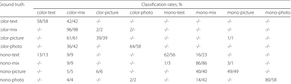
To analyze the classification accuracy of our method, we use the same data set from Hewlett-Packard (HP) as in [1]. The data was carefully selected by HP engineers to include a wide variety of difficult-to-classify scenarios. The entire image database is randomly divided into two equally sized sets, one used for training and the other for testing. All decision parameters are trained using the training set, while all the experimental results are obtained using the test set. These results are summarized in Tables 3, 4, and 5. Each entry in the tables represents the empirical condi-tional probabilityP (classification result | ground truth) for the test data set. These tables allow us to separately dis-cuss the contributions to the overall performance of our proposed new features and of our proposed new overall classification strategy.

In Table 3, we give the classification rates, in percent, for the hard-decision tree classifier of [1] and Fig. 1a. Each entry in the table is of the form “A/B” where A is the clas-sification rate using the features proposed in the present paper, and B is the classification rate using the features from [1].

We observe that the features proposed in the present paper cause a reduction of the classification accura-cies for text, mix, and photo documents. This is due to the fact that our features avoid vertical computa-tions while the ones in [1] do not. However, thanks to our design of halftone noise triplets3, our new features

Table 2The average running time and the memory requirement for [1] and this work

Method Average running time Memory requirement

The proposed 0.268 s one strip

Table 3Classification rates for the test data set, using the hard-decision tree classifier of Fig. 1a [1]

Ground truth Classification rates, %

color-text color-mix color-picture color-photo mono-text mono-mix mono-picture mono-photo

color-text 58/60 42/40 -/- 1/- -/- -/- -/-

-/-color-mix -/1 98/98 2/1 -/- -/- -/- -/-

-/-color-picture -/- 61/58 39/38 -/3 -/- -/- 1/1

-/-color-photo -/- 42/36 -/- 58/64 -/- -/- -/-

-/-mono-text 13/14 9/6 -/- -/- 56/65 23/15 -/-

-/-mono-mix -/- 9/5 -/- -/- 3/1 86/89 1/5

-/-mono-picture -/- 5/6 6/1 -/- -/- 40/63 49/30

-/-mono-photo -/- 4/5 -/- 2/1 -/- 42/26 -/2 58/66

Each entry in the table is “A/B” where A and B are the classification percentages, respectively, for the feature set proposed in the present paper and for the feature set obtained from [1]

improve the correct classification rates of picture doc-uments. Specifically, features from [1] have 2, 6, 9, 3, and 8 % higher classification accuracies for color-text, color-photo, mono-text, mono-mix, and mono-photo, respectively; while our proposed features have the cor-rect classification gain of 1 and 19 % for color-picture and mono-picture, respectively.

In Table 4, we present the classification results for our proposed hard/soft classification strategy of Fig. 3a. These are compared to the hard-decision tree classifier of Fig. 1a and [1], applied to the features described in the present paper. Two experimental results are shown in each entry of the tables using the format“A/B", where A is the clas-sification percentage using the hybrid hard/soft classifier proposed in this paper, and B is the classification percent-age for the hard-decision tree classifier.

We observe that, at the expense of a very slight reduc-tion in the correct classificareduc-tion rate for color-mix images, our new classification strategy results in significant improvements of the correct classification rates of photo

and mono-text documents. Specifically, the hard decision method has 2 % correct classification gain for color-mix, while the proposed hybrid hard/soft method has 6, 6, and 22 % gains for color-photo, mono-text, and mono-photo, respectively.

To compare the overall performance of our new clas-sifier (i.e., the new features and the new classification strategy) to that of the classifier in [1], we can compare the first number in each cell of Table 4 with the second number in the corresponding cell of Table 3. Six out of the eight correct classification rate numbers are very similar between the two algorithms. The two numbers that are more than three percentage points apart are the correct classification rates for mono-picture and mono-photo: the former is 49 % for our algorithm and 30 % for the algo-rithm in [1], and the latter is 80 % for our algoalgo-rithm and 66 % for the algorithm in [1].

Figure 7 shows two mono-photo images that were mis-classified by the hard decision method, but correctly clas-sified by our proposed hybrid hard/soft decision method.

Table 4Classification rates for the test data set, using the proposed features

Ground truth Classification rates, %

color-text color-mix clor-picture color-photo mono-text mono-mix mono-picture mono-photo

color-text 58/58 42/42 -/- -/- -/- -/- -/-

-/-color-mix -/- 96/98 2/2 2/- -/- -/- -/-

-/-color-picture -/- 61/61 39/39 -/- -/- -/- 1/1

-/-color-photo -/- 36/42 -/- 64/58 -/- -/- -/-

-/-mono-text 13/13 9/9 -/- -/- 62/56 16/23 -/-

-/-mono-mix -/- 9/9 -/- -/- 1/3 86/86 3/1

-/-mono-picture -/- 5/5 6/6 -/- -/- 40/40 49/49

-/-mono-photo -/- 4/4 -/- 2/2 -/- 14/42 -/- 80/58

Fig. 7Two examples (a,b) that were misclassified by the hard decision classifier, but classified correctly by the hybrid hard/soft decision method

The hard decision classifier misclassifies them as mix early on in the decision tree (see Fig. 1) and does not even get to compute the roughness feature score which greatly differs between mono-photo and the other mono originals. On the other hand, the hybrid hard/soft deci-sion method keeps these images from being misclassified since the roughness feature score is considered simul-taneously with the other features in the classification process.

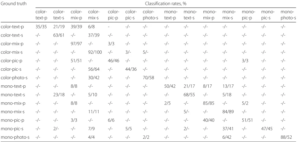
The classification results that include the periodic-vs-stochastic classification, are presented in Table 5, for both the hard-decision classifier of Fig. 1b and the hard/soft-decision classifier of Fig. 3b. Observe that our periodic halftone detector works without error for almost every mode. A notable exception is the text mode. Several odic halftone text documents contain very limited peri-odic halftone regions as illustrated in Fig. 8, and hence our algorithm misclassifies them as stochastic halftone

documents. The overall accuracy of our halftone classi-fier on the test suite is 97 %. The halftone classiclassi-fier, in its current form, is computationally heavy compared to the rest of the algorithm. With the halftone classification node added, the average per-image processing time increases from 0.268 to 0.963 s on an Intel(R) Core(TM) i7-4770 3.40 GHz desktop.

The color-vs-mono classification task has been addressed in numerous patents many of which use ideas similar to ours [20–39]. As we mention in [1], the mixed raster content (MRC) model [40] could be used to improve our text-vs-nontext classifier as the expense of prohibitive complexity. Similarly unaffordable complexity would accompany improvements to our text/mix-vs-picture/photo classifier based on, for example, [41]. Halftone detection techniques that may be used for separating pictures from photos [42–46] are discussed in [1]. Those of them that have low enough complexity to be

Table 5Classification rates for the test data set, using the proposed features

Ground truth Classification rates, %

color- color- color- color- color- color- color- mono- mono- mono- mono- mono- mono- mono-text-p text-s mix-p mix-s pic-p pic-s photo-s text-p text-s mix-p mix-s pic-p pic-s photo-s

color-text-p 35/35 21/19 39/39 6/8 - -/- -/- -/- -/- -/- -/- -/- -/-

-/-color-text-s -/- 63/61 -/- 37/39 -/- -/- -/- -/- -/- -/- -/- -/- -/-

-/-color-mix-p -/- -/- 97/97 -/- 3/3 -/- -/- -/- -/- -/- -/- -/- -/-

-/-color-mix-s -/- -/- -/- 92/100 -/- 3/- 5/- -/- -/- -/- -/- -/- -/-

-/-color-pic-p -/- -/- 51/51 -/- 46/46 -/- -/- -/- -/- -/- -/- 3/3 -/-

-/-color-pic-s -/- -/- -/- 56/64 -/- 44/36 -/- -/- -/- -/- -/- -/- -/-

-/-color-photo-s -/- -/- -/- 30/42 -/- -/- 70/58 -/- -/- -/- -/- -/- -/-

-/-mono-text-p -/- -/- 8/8 -/- -/- -/- -/- 50/42 21/17 8/17 13/17 -/- -/-

-/-mono-text-s -/- 23/18 -/- 5/10 -/- -/- -/- -/- 68/55 -/- 5/18 -/- -/-

-/-mono-mix-p -/- -/- 8/8 -/- -/- -/- -/- 2/5 -/- 85/85 -/- 5/2 -/-

-/-mono-mix-s -/- -/- -/- 11/11 -/- -/- -/- -/- 5/- -/- 84/89 -/- -/-

-/-mono-pic-p -/- -/- 3/3 -/- 6/6 -/- -/- -/- -/- 40/40 -/- 51/51 -/-

-/-mono-pic-s -/- 2/- -/- 7/9 -/- 5/5 -/- -/- 2/- -/- 37/41 -/- 47/45

-/-mono-photo-s -/- -/- -/- 4/4 -/- -/- 2/2 -/- -/- -/- 6/42 -/- -/- 88/52

Fig. 8 aAn example of text document that contains very limited periodic halftone region.bZoomed-in version of the periodic region ofa

appropriate for our application, are outperformed by our method, as shown in [1].

There is also a vast amount of literature on construct-ing classifiers [8–17]. There exist a myriad methods to partition our multidimensional feature space into several classification regions. In designing the overall structure of our algorithm, there were two things we were striving for, besides low complexity and high accuracy:

• Small number of parameters, in order to avoid overfitting.

• Structural simplicity, so that the algorithm is easy to understand and implement. This is greatly helped by the modular structure of the algorithm where each module only involves one or two features and is mainly responsible for the classification into two or three subclasses.

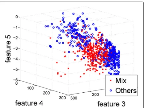
Interestingly, despite the relative simplicity of our algo-rithm, both conceptual and computational, at the same time it is able to produce very complex decision bound-aries, as illustrated by Fig. 9. This figure shows a 3D scatter plot of three features (luminance variability score, text edge score, and unnaturalness score) for the images that our algorithms classifies as mix (red X’s) and for the images that our algorithm classifies as non-mix (blue O’s).

5 Conclusions

In this paper, we have presented an algorithm to auto-matically classify documents into a set of categories. This algorithm could be used as a copy mode selector uti-lized to improve the copy quality and increase the copy rate. Our method retains some of the features of the method in [1], but both extends the number of classes to identify periodic halftone and includes several important

modifications both in the feature extraction stage and in the classification strategy. As compared to [1], the classi-fication rate is improved by up to 22 % while the running time and memory requirements are saved for 18 and 50 %, respectively.

Endnotes

1_{All running times in this paragraph are for}

classifica-tions that use the feature set developed in the present paper.

2_{This value of T makes Eq. (2) redundant, as it then}

follows from Eq. (3).

3_{Halftone noise triplets are used to alleviate false text}

edge detection from halftone noise.

Acknowledgements

This work is partly supported by Ministry of Science and Technology of Taiwan under Grant MOST103-2221-E-011-105 and MOST104-2221-E-011-091-MY2.

Authors’ contributions

KH proposed the framework of this work and drafted the manuscript; WH, YC, and CH carried out the algorithm studies, participated in the simulation, and helped draft the manuscript. PL participated in the discussion, corrected the English errors, and helped polish the manuscript. All authors read and approved the final manuscript.

Competing interests

The authors declare that they have no competing interests.

Received: 9 July 2015 Accepted: 20 September 2016

References

1. X Dong, K-L Hua, P Majewicz, G McNutt, CA Bouman, JP Allebach, I Pollak, Document page classification algorithms in low-end copy pipeline. J. Electron. Imaging.17(4), 043011–043011 (2008)

2. W Zhang, X Tang, T Yoshida, Tesc: An approach to text classification using semi-supervised clustering. Knowl.-Based Syst.75, 152–160 (2015) 3. H Cheng, CA Bouman, Document compression using rate-distortion

optimized segmentation. J. Electron. Imaging.10(2), 460–474 (2001) 4. RL de Queiroz, inImage Processing, 1999. ICIP 99. Proceedings. 1999

International Conference On. Compression of compound documents, vol. 1 (IEEE, 1999), pp. 209–213

5. SV Revankar, Z Fan, inPhotonics West 2001-Electronic Imaging. Picture, graphics, and text classification of document image regions (International Society for Optics and Photonics, 2000), pp. 224–228

6. SJ Simske, SC Baggs, inProceedings of the 2004 ACM Symposium on Document Engineering. Digital capture for automated scanner workflows (ACM, 2004), pp. 171–177

7. W Wang, I Pollak, T-S Wong, CA Bouman, MP Harper, JM Siskind, Hierarchical stochastic image grammars for classification and segmentation. IEEE Trans. Image Process.15(10), 3033–3052 (2006) 8. T Hastie, R Tibshirani, J Friedman, J Franklin, The elements of statistical

learning: data mining, inference and prediction. Math Intell.27(2), 83–85 (2005)

9. RO Duda, PE Hart, DG Stork,Pattern classification, (2000) 10. CM Bishop, et al,Pattern Recognition and Machine Learning, vol. 4.

(Springer, New York, 2006)

11. J Kumar, J Pillai, D Doermann, inDocument Analysis and Recognition (ICDAR), 2011 International Conference On. Document image classification and labeling using multiple instance learning (IEEE, 2011), pp. 1059–1063 12. L Han, J Yu, J Chen, K Zheng, J Luo, Research and application of a method

for real estate document image classification. J. Inf. Comput. Sci.6, 1617–1624 (2012)

13. M-R Bouguelia, Y Belaid, A Belaïd, inImage Processing (ICIP), 2013 20th IEEE International Conference On. Document image and zone classification through incremental learning (IEEE, 2013), pp. 4230–4234

14. AGS de Herrera, D Markonis, H Müller, inMedical Content-Based Retrieval for Clinical Decision Support. Bag-of-colors for biomedical document image classification (Springer, 2013), pp. 110–121

15. L Kang, J Kumar, P Ye, Y Li, D Doermann, inPattern Recognition (ICPR), 2014 22nd International Conference On. Convolutional neural networks for document image classification (IEEE, 2014), pp. 3168–3172

16. AW Harley, A Ufkes, KG Derpanis, Evaluation of deep convolutional nets for document image classification and retrieval (2015). arXiv preprint arXiv:1502.07058

17. J Kumar, P Ye, D Doermann, Structural similarity for document image classification and retrieval. Pattern Recogn. Lett.43, 119–126 (2014) 18. SC Hidayati, C-H Hsu, S-W Sun, W-H Cheng, K-L Hua, inInternational

Conference on Multimedia & Expo (ICME) Workshop. An efficient algorithm for periodic halftone identification (IEEE, 2015)

19. S Kim, S Youn, S Baek, C Lee, in2015 IEEE 4th Global Conference on Consumer Electronics (GCCE). Document classification for copy-mode decision (IEEE, 2015), pp. 517–518

20. K Nagata, Device for judging the type of color of a document. Google Patents. US Patent 5,282,026 (1994)

21. H Koizumi, K Kouno, Y Sorimachi, Y Suzuki, Y Awata, Image recognition apparatus for judging between monochromic and color originals. Google Patents. US Patent 5,287,204 (1994)

22. Z Fan, Y Zhang, ME Banton, Multi-resolution neutral color detection. Google Patents. US Patent 6,249,592 (2001)

23. Y Hirota, K Toyama, S Imaizumi, H Hashimoto, K Ishiguro, Image processing apparatus, image forming apparatus and color image determination method thereof. Google Patents. US Patent 7,177,462 (2007)

24. W-H Hsieh, C-H Shih, I-C Teng, Method of determining color composition of an image. Google Patents. US Patent 7,308,137 (2007)

25. J Shishizuka, Method and apparatus for processing image. Google Patents. US Patent 5,786,906 (1998)

26. Y Hirota, K Toyama, S Imaizumi, H Hashimoto, K Ishiguro, Image processing apparatus, image forming apparatus and color image determination method thereof. Google Patents. US Patent 7,319,786 (2008) 27. Y Hirota, K Toyama, T Nabeshima, Image forming apparatus for

distinguishing between types of color and monochromatic documents. Google Patents. US Patent 6,118,895 (2000)

28. K Murai, N Kasahara, K Hashimoto, Color image processing apparatus. Google Patents. US Patent 5,032,904 (1991)

29. H Tanaka, Image determining apparatus capable of properly determining image and image forming apparatus utilizing the same. Google Patents. US Patent 6,900,902 (2005)

30. K Hara, Image processing apparatus and method, and image processing system. Google Patents. US Patent 6,804,033 (2004)

31. K Kanamori, Image processing method, Image processing apparatus and image forming apparatus. Google Patents. US Patent 6,643,397 (2003) 32. H Kawano, H Yamamoto, Image discriminating apparatus. Google

Patents. US Patent 6,240,203 (2001)

33. H Kawano, Color type determining device. Google Patents. US Patent 6,256,112 (2001)

34. K Yamamoto, Y Matsui, H Matsuo, Image processing apparatus. Google Patents. US Patent 5,734,758 (1998)

35. J Bares, TW Jacobs, Detecting process neutral colors. Google Patents. US Patent 6,972,866 (2005)

36. JC Handley, Y-w Lin, Neutral pixel detection using color space feature vectors wherein one color space coordinate represents lightness. Google Patents. US Patent 7,116,443 (2006)

37. D Horie, N Okisu, Color discrimination apparatus and method. Google Patents. US Patent 6,480,624 (2002)

38. MR Grosso, CD Woodward, Automatic detection of black and white pages in a color document stream. Google Patents. US Patent 6,718,878 (2004) 39. H Kanno, T Sawada, Color image-forming apparatus capable of

discriminating the colors of the original image. Google Patents. US Patent 6,504,628 (2003)

40. RL de Queiroz, RR Buckley, M Xu, inProc. SPIE. Mixed raster content (mrc) model for compound image compression, vol. 3653, (1998),

pp. 1106–1117

41. Z Fan, Image type classification using color discreteness features. Google Patents. US Patent 6,996,277 (2006)

42. X Li, ME Meyers, KT Francis, Image segmentation apparatus and method. Google Patents. US Patent 6,389,164 (2002)

43. RL Triplett, RJ Clark, J-N Shiau, Method and system for classifying and processing of pixels of image data. Google Patents. US Patent 6,347,153 (2002)

44. SA Schweid, J-N Shiau, Method and system for classifying and processing of pixels of image data. Google Patents. US Patent 6,549,658 (2003) 45. Y-w Lin, AF Calarco, Image processing apparatus using approximate auto

correlation function to detect the frequency of half-tone image data. Google Patents. US Patent 4,811,115 (1989)