Compound optimal control of harmonic drive considering hysteresis characteristic

https://doi.org/10.5194/ms-10-383-2019

© Author(s) 2019. This work is distributed under the Creative Commons Attribution 4.0 License.

Compound optimal control of harmonic drive

considering hysteresis characteristic

Quan Lu1, Tieqiang Gang1, Guangbo Hao2, and Lijie Chen1 1_{School of Aerospace Engineering, Xiamen University, Xiamen, 361005, China}

2_{School of Engineering, University College Cork, Cork, Ireland}

Correspondence:Tieqian Gang ([email protected]) and Lijie Chen ([email protected])

Received: 4 January 2019 – Revised: 23 January 2019 – Accepted: 3 June 2019 – Published: 22 July 2019 Abstract. Hysteresis behavior widely exists in the transmission process of harmonic drives. Eliminating the hysteresis effect is highly desired in the high-precision mechanical transmission, which results in challenges in the control design. This paper aims to improve the tracking accuracy of the motor-harmonic drive serial system. Firstly, a modified Bouc-Wen model based on uniform smooth approximating function is applied to describe the hysteresis behavior of the harmonic drive. By using coordinate transformation and accurate state feedback linearization, we then obtain the mathematical model of the serial system of the motor-harmonic drive. Finally, the reference trajectory is tracked by a compound optimal controller that is based on a linear quadratic regulator. Simulation results show that compared with the disturbance observer-based control (DOBC) using a linear observer, the new compound optimal controller in this paper presents a smoother control signal with the elimination of large amount of high-frequency oscillations. Furthermore, the relative error in the steady state tracking tends to approach to zero and no cyclic fluctuations appears. With the employing of optimal control, the output of the harmonic drive can trace more complex trajectory.

1 Introduction

For an ideal transmission system, the phase diagram of the system state established by the input torque and output dis-placement should be a monotonic curve regardless of loading history. In other words, there should be a one-to-one corre-spondence between the output displacement and input torque of the system. In fact, hysteresis phenomena are widely rec-ognized in the electromechanical transmission systems. Hys-teresis generally means that the current state of the system depends not only on the input at the moment, but also de-pends on the history of input values, i.e. path-dependent pro-cesses (Mayergoyz et al., 2003; Bertotti et al., 1998), which results in lots of control difficulties.

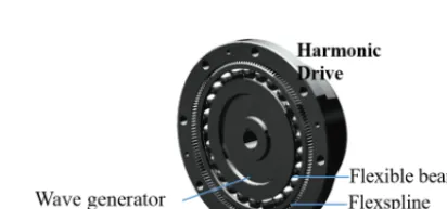
With the development of aerospace industries, as a new transmission system, the servo motor-harmonic drive serial system is widely used in transmission mechanisms of rockets and satellites. However, due to the nonlinear contact friction between the flexspline and the circular spline (as shown in Fig. 1), together with the viscous friction of the flexible bear-ing, transmission hysteresis characteristics exist in the servo

Figure 1.Structures of harmonic drive.

motor-harmonic drive serial system. For example, for a ba-sic transmission unit of a robot arm, these inherent nonlinear properties will result in serious hysteresis feature of the trans-mission system and adversely affect the motion precision of the robot arm. This paper focuses on the control of such a harmonic drive system with hysteresis characteristic.

spe-Figure 2.Servo Motor-Harmonic Drive Serial System.θm is the rotation angle of the motor rotor,θlthe rotation angle on the output port of the harmonic drive, andτmthe output torque of servo motor.

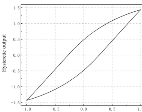
Figure 3.Example of a Hysteresis Loop.

cific hysteresis behaviors for harmonic drives in which de-tailed experimental data are required to define. Kircanski et al. (1997) designed an experiment, in which two torque sen-sors were set up at both the input port of the motor and the output port of the harmonic drive, and the input torque curve of the motor was controlled to be a harmonic wave with a fixed maximum magnitude. It was found in the experiment that when the input torque returned to zero after several peri-ods, the output of the harmonic drive was not zero. Dhaouadi et al. (2003) also conducted experimental testing to reveal the hysteresis, where the output port of the harmonic drive was locked and a periodic torque was forcibly exerted on the motor side. The experimental result showed that the hystere-sis characteristic is insensitive to the input frequency when the input toque maintains a constant magnitude. The advan-tage of this experimental scheme lies in the ability of secure testing of the high-frequency input responses. Both the ex-perimental results provide us with basis on the study of the hysteresis model so that we can select the corresponding pa-rameters to establish an optimal control method with a higher precision for a hysteresis system.

In literatures, there are many existing mathematical mod-els proposed to describe hysteresis, such as LuGre model (Kamlah and Jiang, 1999), Preisach model (Song et al., 2005), Duhem model (Lee and Royston, 2000), Maxwell model (Huang and Chiu, 2009) and Bouc-Wen model (Zhu et al., 2014). Among these models, the Bouc-Wen model is a classical and most widely used one. However, this model

is not differentiable everywhere, which will be improved in the present paper by using uniform smooth approximating function.

Meanwhile, there are also various control theories that can be used to compensate for hysteresis issues, including PID (proportional–integral–derivative) control, feed-forward controller, adaptive control, and sliding mode control.

PID controller does not depend on the specific structure of the controlled object, which makes it theoretically capable of solving the hysteresis problem. However, for the system with sharp changes, PID controller cannot compensate for the hysteresis torque in real time. Different from PID control, the feed-forward controller requires sophisticated modeling and precise parameters. Considering this, An et al. (1989) introduced the feed-forward control into a PD (proportional-derivative) control and used this compound method to control the robotic arm equipped with a harmonic drive.

Adaptive control is the most widely used method for hys-teresis compensations. Many newly emerging control theo-ries, such as fuzzy theory, internal model principle and neural network, have been utilized in combination with the adaptive control. For an unknown nonlinear friction model, Tadayoni et al. (2011) approximated the friction torque by using the wavelet network and fuzzy structure. However, implement-ing these compound controllers requires the control unit to provide certain challenging computing ability and data stor-age capacity. Under current technical conditions with ordi-nary industrial control chips, it is difficult to satisfy these re-quirements to implement such a compound control.

Sliding mode controller can compensate for the hystere-sis in real time with high precision. Moreover, by using the sliding mode controller we can achieve the same control re-sult at a relatively low cost. He et al. (2009) used a LuGre model as the controlled object of a sliding mode controller, with a successful simulation demonstration. Unfortunately, for the harmonic drive in engineering applications, the tremor caused by the high-frequency switching signals in the sliding mode controller can excite high-order unmodeled dynamics of the system. This consequence will seriously jeopardize the transmission precision of the system (Bandyopadhyay et al., 2015). In summary, these controllers are not suitable for a motor-harmonic drive electromechanical transmission sys-tem.

controller using numerical simulation, by comparing with the distribute observer based control (DOBC). Conclusions are drawn in Sec. 6.

2 Mathematical modeling of hysteresis

characteristic of motor-harmonic drive system

The motor-harmonic drive system has two degrees of free-dom, which are defined by the rotation angle of the motor rotor,θm, and the rotation angle on the output port of the har-monic drive,θl, as shown in Fig. 2. The Lagrange equations of the transmission system can be written as follows:

              

Jmθ¨m+Bmθ˙m+ K N

_θ m N −θl

+ 1

Nq=τm, Jlθ¨l+Blθ˙l−K

_θ m N −θl

−q=0,

˙

q+a ˙ θm N − ˙θl

q−A _θ˙

m N − ˙θl

=0,

(1)

whereJmandJlare the inertia moment of the moving part of the motor and the inertia moment of the loading end, respec-tively,Kthe torsional stiffness between the input and output ports of the harmonic drive, andN the transmission ratio.

With the third nonlinear differential formula in Eq. (1), one can obtain the hysteresis torqueq. This formula is the special form of the standard Bouc-Wen model with particular param-eters of n=1 and β=0 (Gandhi et al., 2001). The fitting results of experimental data fromIkhouane et al. (2007) indi-cate that the model with only two positive parameters,aand A, can already well describe the hysteresis in the harmonic drive.BmandBlin Eq. (1) represent viscous damping coeffi-cients inside the motor and harmonic drive, respectively. The two parameters are acquired according to the experimental data.

If we define the state variable vector as x= [x1, x2, x3, x4, x5]T = [ ˙θm, θm,θ˙l, θl, q]T, Eq. (1) can be rewritten into the form of state space as below:

                   ˙

x1= − Bm

Jm x1−

K

JmN2 x2+

K

JmN x4−

1

JmN x5+u,

˙

x2=x1,

˙

x3= Bl Jl

x3− K Jl

x4+ K JlN

x2+ 1 Jl

x5,

˙

x4=x3,

˙

x5= −a

x1 N −x3

x5+A

x₁ N −x3

.

(2)

The compact form of Eq. (2) is:

_˙

x=f(x)+g(x)u,

y=h(x)=[0,0,0,1,0]x. (3) The system described by Eq. (3) is a typical nonlinear affine single-input single-output (SISO) system (Dierks et al., 2010), in which the system input is the motor torque u and the output is the angular displacement θl of the output

port of the harmonic drive. The absolute value function in Eq. (3) keeps us from calculating the analytic solution of its Jacobian matrix. So in the present paper, uniformly smooth approximating functions are used to approximate the abso-lute value function (for the detailed deduction and proof pro-cess, refer to Long-quan et al., 2015), then we have:

f(x)=

          

−Bm

Jm x1−

K JmN2

x2+ K JmN

x4− 1 JmN

x5 x1

−Bl

Jl x3−

K Jl

x4+ K JlN

x2+ 1 Jl

x5

˙

θl

−aµln e 1 µ _x 1

N−x3

+e−

1

µ _x

1

N−x3

q+A x₁

N −x3            , (4)

whereµ=0.001 andg(x)=[1,0,0,0,0]T. All the system state variables exceptqare measurable, andqis a compound function of other state variables. Until this step, one obtain a controllable dynamic model. By measuring state variables of this model, we can create feedback channels to compen-sate the system for hysteresis torque directly or indirectly. In the following, we will discuss the design of a reasonable controller so that the system outputθlcan track the reference trajectoryrin a desired way.

3 Precise State Feedback Linearization and Optimal Controller Design

For the classical optimal control, we need to firstly determine the objective function of the optimal problem. Suppose that the initial conditions of the nonlinear affine system isx0= [0,0,0,0,0]T, the terminal time tfis fixed and the terminal statex(tf) is free. Then, the objective function (Anderson et al., 2007) that needs to be minimized is constructed as:

J=1

2 Z _h

M(r−y)2+Ru2 i

dt, (5)

system outputy=h(x) are:                                ˙

y=∂h(x)

∂t = ∂h(x)

∂xT ∂x

∂t

=∂h(x)

∂xT

f(x)+g(x)u₌

Lfh(x)+Lgh(x)u,

¨

y=∂y˙

∂t = ∂y˙

∂xT ∂x

∂t = ∂y˙

∂xT

f(x)+g(x)u

=L2_fh(x)+LgLfh(x)u, . . .

y(n)=∂y

(n−1) ∂xT

∂x

∂t =

∂Ln_f−1h(x) ∂xT

f(x)+g(x)u

=Ln_fh(x)+LgLnf−1h(x)u.

(6)

Substituting Eqs. (3)–(5) into the Eq. (6) and expanding the results, it can be observed that the right-hand sides of the first three equations do not explicitly contain u, andLgL3fh(x) contained in the fourth equation is the first nonzero poly-nomial. Therefore, it is unnecessary to take more than fifth-order derivations The results in Eq. (6) are thus simplified as follows:                                           

z1=y=x4, z2= ˙y=x3, z3= ¨y= −

Bl Jl

x3− K

Jl x4+

K

JlN x2+

1

Jl x5, z4=y(3)=

K JlN

x1

±Bl

Jl

−Bl

Jl x3−

K Jl

x4+ K JlN

x2+ 1 Jl x5 −K Jl x3+

1 Jl

−aµln e 1 µ _x 1

N−x3

+e−

1

µ _x

1

N−x3

q

+Ax1 N −x3

,

y(4)=H(x)+G(x)u,

(7)

whereH(x) equals to:

H(x)=



 K JlN

+ A

JlN

− 1

JlN aqe

1

µ _x

1

N−x3

−e−

1

µ _x

1

N−x3

e 1 µ _x 1

N−x3

+e−

1

µ _x

1

N−x3

    

−Bm

Jm x1−

K

JmN2 x2+ K

JmN x4−

1 JmN

x5 

 −

BlK J_l2Nx1

+



 B_l2 J_l2

−K

Jl

+ABl

Jl

− 1

Jl aq−e

1

µ _x

1

N−x3

+e−

1

µ _x

1

N−x3

e 1 µ _x 1

N−x3

+e−

1

µ _x

1

N−x3     

−Bl

Jl x3−

K Jl

x4

+ K

JlN x2+

1 Jl x5   +

BlK J_l2 x3

+

( Bl J_l2

− 1 Jl aµln e 1 µ _x 1

N−x3

+e−

1

µ _x

1

N−x3

)      A

Nx1−Ax3− aµqln e 1 µ _x 1

N−x3

+e−

1

µ _x

1

N−x3

     ,

andG(x) is:

G(x)= K

JlN

+ A

JlN

− 1

JlN aqe

1

µ _x

1

N−x3

−e−

1

µ _x

1

N−x3

e 1 µ _x 1

N−x3

+e−

1

µ _x

1

N−x3

. (8)

It can be seen that for a nonlinear affine system shown in Eq. (3), if a nonlinear state feedback function, such as u= 1

G(x)[r−H(x)], is appropriately added, the system will degenerate into a quadratic integration system:

y(4)=r. (9)

G(x) is not zero around the initial statex0= [0,0,0,0,0]T of the transmission system, which means that the precise state feedback linearization is nonsingular around the ini-tial pointx0. Based on Eq. (10), we can design an optimal controller to track the trajectory. Assuming that the objective function of the system is:

J=1

2 Z _h

M(r−z1)2+Ru20 i

dt. (10)

Using the Pontryagin’s minimum principle, the Hamiltonian function is obtained:

H=1

2M(r−z1) 2₊1

2Ru 2_+λ

−1

Rλ4and the following equations:                                            ∂H ∂z1

= − ˙λ1= −M(r−z1), ∂H

∂z2

= − ˙λ2=λ1, ∂H

∂z3

= − ˙λ3=λ2, ∂H

∂λ1

= ˙z1=z2, ∂H

∂λ2

= ˙z2=z3, ∂H

∂λ3

= ˙z3=z4, ∂H

∂λ4

= ˙z4=u0= − 1 Rλ4.

(12)

The boundary conditions are:

λ=



  

λ1(tf) λ2(tf) λ3(tf) λ4(tf)     =     0 0 0 0     . (13)

Here, the control signalu0is determined by the co-state vari-ableλ, reference inputrand system feedbackz1. It is clear that the control signal is independent of the actual structure of the object system. Therefore, by using the following con-trol signal

u= 1

G(x)[u0−H(x)], (14)

and also substituting Eq. (6) into Eq. (13), we have:

                                                

− ˙λ1= −M(r−θl),

− ˙λ2=λ1,

− ˙λ3=λ2,

− ˙λ4=λ3,

¨

θm= − Bm Jm

x1− K JmN2

x2+ K JmN

x4− 1 JmN

x5

+ 1

G(x)

−1

Rλ4−H(x)

,

˙

θm=x1,

¨

θl= Bl

Jl x3−

K Jl

x4+ K JlN

x2+ 1 Jl

x5,

˙

q= −aµln e 1 µ _x 1

N−x3

+e−

1

µ _x

1

N−x3

x5

+Ax1 N −x3

.

(15)

Equation (16) include both the initial-value and boundary-value constraints, namely a complex boundary boundary-value prob-lem (BVP) in which numerical methods are needed to solve the equations (Shampine et al., 2000; Ascher et al., 1994). In terms of Eq. (16), the simulation system is constructed, as shown in Fig. 4.

The simulation steps of the control system are as follows:

– First, calculate the input signal based on the pre-designed trajectoriesr and Eq. (16). The state variable of the controller is the co-state variableλ.

– Then, using the feedback channel, calculate the nonlin-ear feedback signal by measuring the state variable of the transmission system.

– Finally, combining the output signal of the controller with the nonlinear feedback signal and importing them into the transmission system, obtain the desired trajec-tory at the output of the harmonic drive.

4 Simulations

In order to illustrate the superiority of the new compound controller proposed, in this section, we compare the con-trol performance of the present compound concon-troller with the control method of disturbance observer based control (DOBC) (Yang et al., 2011). The main control idea of DOBC is that the hysteresis torques− 1

JmNq and

1

Jlq are treated as

interferences so as to realize real-time compensation, which makes the resulting system become linear, i.e.:

_˙

x=Ax+Bu+Cd,

y=Dx, (16)

whered=q, and

C=        − 1

JmN

0 0 0

0 0 0 0

0 0 1 Jl

q 0

0 0 0 0       

The observer is defined as:

 



˙

z= −LC(z+Lx)−L(Ax+Bu), bd=z+Lx,

u=Kx(r−x)+Kdbd,

(17)

whereKxandKdare feedback gains. The parameters of the observer are: L=    

40 0 0 0 0 40 0 0 0 0 40 0 0 0 0 40



  

Figure 4.Simplified block diagram of the control system constructed according to Eq. (16).

Table 1. The Inherent Parameters of Harmonic Drive System (Gandhi et al., 2001).

Nominal Parameter Value

Motor Inertia:Jm 2.9×10−4kg m−2

Harmonic Drive Inertia:J_l 1.6×10−4kg m−2 Damping of motor bearing:Bm 1.7×10−4Nm s−1

Inner damping of harmonic drive:Bl 1.3×10−5Nm s−1

Harmonic drive transmission ratio:N 50

Torsional stiffness of flex spline:K 7160 Nm rad−1 Parameter of hysteresis model:A 5.5583×103Nm rad−1 Parameter of hysteresis model:a 3.6721×102Nm rad−1

meet the stability requirement of Kx. For cost function of LQR, we selectR=0.001 and

Q=



  

0 0 0 0 0 0 0 0 0 0 0 0 0 0 0 1000



  

Then, we can obtain the controller’s gains Kx= [−0.1469,−37.2786,−0.2057,863.9319] and Kd= [−0.02,0,−0.2803,0].

For the compound optimal control proposed in this paper, there are only two controllable parameters, namely M and R. We can adjust the two parameters to improve the tracking performance of the control system. The rest of the parameters are listed in the Table 1. Numerical simulations show that the smallerRis, the larger the amplitude of the control signal is. By adjustingM, we can also amplify the control signal. It is also noted that ifRis too small, the numerical method will fail to solve the complex BVP (Eq. 16). However, an optimal allowableR can be found to satisfy the tracking precision. So we chooseM=10 000 andR=0.001. Once the param-eters used in DOBC controller and the compound optimal controller have been confirmed, one can compare their con-trol performances by tracking the same reference trajectory r=1−cos(π t).

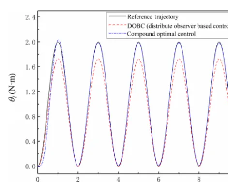
Figure 5.The cosine wave tracking effect of the compound optimal control and DOBC. The tracking curve of the compound optimal control almost overlaps with the reference trajectory.

5 Results and Discussions

The response curves of DOBC and the compound optimal control together with the reference trajectory are shown in Fig. 5. It is observed that the steady-state tracking of the present compound optimal control method is excellent. For DOBC, however, there is always a large tracking error around the peak of the trajectory curve, which means that the track-ing curve cannot follow the reference as desired. This is be-cause the proportional control in DOBC cannot completely get rid of the static error in the closed-loop system.

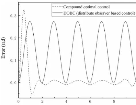
re-Figure 6.Tracking error of DOBC and the compound optimal con-trol.

duces to less than 1 %, while that from DOBC fluctuates peri-odically within 25 %. Therefore, compared with DOBC, the compound optimal control can realize a stable tracking with a much better precision control.

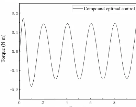
Control signals of DOBC and compound optimal control are shown in Figs. 7 and 8, respectively. As shown in Fig. 7, although DOBC system enters a relatively steady state in general, the control signal is still mixed with a large number of high-frequency components around the peak and valley points of the curve. These high-frequency components result from the linear observer used in estimating hysteresis torque. It is clear that the angular speeds of the harmonic driver and motor change sharply around the peak and valley of the trajectory curve, meaning that the angular accelerations are maximum at the peak and valley points. Meanwhile, it is al-ready known from Eq. (2) that the hysteresis torque is sen-sitive to the angular speed difference between the harmonic drive and the motor. This indicates that the control signal of DOBC inherently contains massive high-frequency compo-nents when tracking complex trajectories. With the increase of the frequency of the reference wave, more high-frequency components can appear. That may be the reason why DOBC is mostly used in the constant speed regulation of the per-manent magnet synchronous motor (PMSM) instead of ac-curate trajectory tracking. In the relevant experimental liter-atures, find similar phenomenon can be found. For example, Lu et al. (2016) built a load DOBC (LDOBC) to estimate the disturbance on load side and realized the trajectory tracking of permanent magnet synchronous machine (PMSM). How-ever, the friction inside the PMSM increases when the motor speed is faster. Their experimental results showed that the high-frequency components in the input signal and output signal increased when the rotate speed increased from 100

Figure 7.The input torque curve of DOBC.

to 2500 rotations per minute. This agrees well with our sim-ulation results.

The control signal of the present compound optimal con-trol in Fig. 8 behaves much smoother and its initial value is zero. Noticeably, the optimal controller eliminates the high-frequency components as seen in DOBC. This resulting con-trol signal requires less bandwidth of the servomotor and lead to more benefit for the stationary-state startup of the servomotor. The control signal of the present controller con-tains no high-frequency components when increasing the fre-quency of the reference cosine wave. Compared with DOBC, the compound optimal control is more adaptive for tracking the complex trajectory with desired precision.

In summary, unlike DOBC which is a closed-loop control based on the real-time feedback, the compound optimal con-troller is an open-loop control. Although the compound op-timal control requires solving the complex BVP equations in advance, the control signal quality and the control effect are much better than those of DOBC. In addition, there are only two parameters (MandR) in the compound optimal control, which can be easily adjusted to meet different requirements. These numerical cases demonstrate that the new com-pound optimal controller presented in this paper has a better comprehensive performance in dealing with hysteresis issue.

6 Conclusions

The present work focuses on the improvement of the track-ing accuracy of the motor-harmonic drive serial system con-sidering the influence of hysteresis torque and a compound optimal control scheme for a harmonic drive has been estab-lished. The main results are summarized as follows.

non-Figure 8.The torque curve of the compound optimal control signal Eq. (15).

differentiable structure of the original system (such as the absolute value function) is approximated by the equivalent smooth function. The new control system is not only benefi-cial to the design of the controller, but also has no singularity around the initial statex0=[0,0,0,0,0]T.

A compound open-loop optimal controller based on a lin-ear quadratic regulator is designed for tracking the expected trajectory of the harmonic drive with hysteresis behavior. In this control method, the quadratic optimal state regula-tor is employed to quantify the whole tracking precision of the control system. In order to get the actual control torque according to the desired trajectory and boundary value, it requires to solve the complex BVP equations in advance. Compared with the traditional control methods, the present compound optimal controller can achieve an optimal perfor-mance and is more adaptive for tracking the complex trajec-tory with desired precision.

Simulation results reveal that when tracking the complex trajectory like cosine wave with similar responding speed, the relative error from DOBC based on linear observer fluctu-ates between 0 % and 25 %. However, for the new compound optimal controller, the relative error of the steady state can be smaller than 1 % and no periodic fluctuation phenomenon ap-pears. In addition, the compound optimal controller can elim-inate the high-frequency components that appear in DOBC. In other words, the control signal curve of the compound op-timal controller is much smoother and more suitable for the torque output of the actual servomotor, than that of DOBC.

Further work is planned on improving the ability of noise resistance and reducing the computational complexity of this new controller. In doing this, we can extend the optimiza-tion problem to the robust control problem where the online optimal control becomes necessary.

Data availability. The authors declare that all data supporting the findings of this study are available within the article or upon request by contact with the corresponding author (see in particular Gandhi, 2001).

Author contributions. QL and TQG conceived the basic idea about the study. QL performed the numerical simulations. QL, LJC, TQG, and GBH wrote, revised and approved the manuscript to-gether.

Competing interests. The authors declare that they have no con-flict of interest.

Financial support. This research has been supported by the Na-tional Natural Science Foundation of China (grant no. 51475396).

Review statement. This paper was edited by Jinguo Liu and re-viewed by Xibin Cao and one anonymous referee.

References

An, C. H., Atkeson, C. G., Griffiths, J. D., and Hollerbach, J. M.: Experimental evaluation of feedforward and com-puted torque control, IEEE T. Robotic Autom., 5, 368–373, https://doi.org/10.1109/70.34773, 1989.

Anderson, B. D. and Moore, J. B.: Optimal control: linear quadratic methods, Courier Corporation, Prentice-Hall, 2007.

Ascher, U. M., Mattheij, R. M., and Russell, R. D.: Numerical solu-tion of boundary value problems for ordinary differential equa-tions, Classics in Applied Mathematics, Society for Industrial and Applied Mathematics, Siam, 13, 1994.

Bandyopadhyay, B. and Patil, M.: Sliding mode con-trol with the reduced-order switching function: an SCB approach, ISPRS Int. Geo.-Inf., 88.5, 1089–1101, https://doi.org/10.1080/00207179.2014.989409, 2015.

Bertotti, G.: Hysteresis in magnetism: for physicists, materials sci-entists, and engineers, Academic press, 1998.

Chiasson, J.: Dynamic feedback linearization of the induc-tion motor, IEEE T. Automat. Contr., 38, 1588–1594, https://doi.org/10.1109/9.241583, 1993.

Dhaouadi, R., Ghorbel, F. H., and Gandhi, P. S.: A new dynamic model of hysteresis in harmonic drives, IEEE T. Ind. Electron., 50, 1165–1171, https://doi.org/10.1109/TIE.2003.819661, 2003. Dierks, T. and Jagannathan S.: Optimal control of affine nonlin-ear continuous-time systems, Proceedings of the 2010 American Control Conference, Baltimore, MD, USA, 30 June–2 July 2010, 1568–1573, https://doi.org/10.1109/ACC.2010.5531586, 2010. Gandhi, P. S.: Modeling and control of nonlinear transmission

at-tributes in harmonic drive systems, Dissertation, Rice University, 2001.

Computation Technology and Automation, 2, 826–829, https://doi.org/10.1109/ICICTA.2009.435, 2009.

Huang, S. J. and Chiu, C. M.: Optimal LuGre friction model iden-tification based on genetic algorithm and sliding mode control of a piezoelectric-actuating table, T. I. Meas. Control, 31, 181–203, https://doi.org/10.1177/0142331208093938, 2009.

Ikhouane, F. and Rodellar J.: Systems with hysteresis: analysis, identification and control using the Bouc-Wen model, John Wi-ley & Sons, 2007.

Kamlah, M. and Jiang Q., A constitutive model for ferroelectric PZT ceramics under uniaxial loading, Smart Mater. Struct., 8, 441, https://doi.org/10.1088/0964-1726/8/4/302, 1999.

Kircanski, N. M. and Goldenberg, A. A.: An experimental study of nonlinear stiffness, hysteresis, and friction effects in robot joints with harmonic drives and torque sensors, Int. J. Robot Res., 16, 214–239, https://doi.org/10.1177/027836499701600207, 1997. Lee, S.-H., and Royston, T. J.: Modeling piezoceramic transducer

hysteresis in the structural vibration control problem, J. Acoust. Soc. Am., 108, 2843–2855, https://doi.org/10.1121/1.1323464, 2000.

Lee, D., Kim, H. J., and Shankar, S.: Feedback linearization vs. adaptive sliding mode control for a quadrotor helicopter, Int. J. Control Autom., 7, 419–428, https://doi.org/10.1007/s12555-009-0311-8, 2009.

Li, S., Yang, J., Chen, W. H., and Chen, X.: Disturbance observer-based control: methods and applications, CRC press, 2014. Long-quan, Y.: Uniform Smooth Approximating Functions for

Ab-solute Value Function, Mathematics in Practice and Theory, 45, 250–255, 2015.

Mayergoyz, I. D.: Mathematical models of hysteresis and their ap-plications, Academic Press, 2003.

Shampine, L. F., Reichelt, M. W., and Kierzenka, J.: Solving bound-ary value problems for ordinbound-ary differential equations in MAT-LAB with bvp4c, available at: http://www.mathworks.com, last access: 9 July 2019.

Song, G., Zhao J. Zhou, X., and De Abreu-Garcia, J. A.: Tracking control of a piezoceramic actuator with hysteresis compensation using inverse Preisach model, IEEE-ASME T. Mech., 10, 198– 209, https://doi.org/10.1109/TMECH.2005.844708, 2005. Tadayoni, A., Xie W. F., and Gordon B. W.: Adaptive control of

har-monic drive with parameter varying friction using structurally dynamic wavelet network, Int. J. Control Autom., 9, 50–59, https://doi.org/10.1007/s12555-011-0107-5, 2011.

Xiaoquan, L., Heyun, L., and Junlin, H.: Load disturbance observer-based control method for sensorless PMSM drive, IET Electr. Power App., 10, 735–743, https://doi.org/10.1049/iet-epa.2015.0550, 2016.

Yang, J., Zolotas, A., Chen, W. H., Michail, K., and Li, S.: Ro-bust control of nonlinear MAGLEV suspension system with mis-matched uncertainties via DOBC approach, ISA T., 50, 389–396, https://doi.org/10.1016/j.isatra.2011.01.006, 2011.