https://doi.org/10.5194/ms-10-393-2019
© Author(s) 2019. This work is distributed under the Creative Commons Attribution 4.0 License.
Design of experiment-based tolerance synthesis for a
lock-or-release mechanism of the Chinese Space Station
Microgravity Platform
Jian Ding1, Jinguo Liu1, Lu Zhang2, Haitao Luo1, Rongpeng Zhang1, Guangbo Hao1,3, and Yuwang Liu1 1State Key Laboratory of Robotics, Shenyang Institute of Automation,
Chinese Academy of Sciences, Shenyang, China
2Key Laboratory of Space Utilization, Technology and Engineering Center for space Utilization, Chinese Academy of Sciences, Beijing, China
3School of Engineering-Electrical and Electronic Engineering, University College Cork, Cork, Ireland
Correspondence:Jinguo Liu ([email protected])
Received: 14 March 2019 – Revised: 22 May 2019 – Accepted: 28 June 2019 – Published: 31 July 2019
Abstract. This paper deals with the tolerance synthesis with the application for a typical Lock-or-Release (L/R) mechanism, used for Chinese Space Station Microgravity Platform (SSMP). The L/R mechanism is utilized to lock the SSMP maintaining space position during the launching stage, and to release the SSMP automatically during on-orbit stage. Manufacturing accuracy of L/R mechanism presents direct influence on its kinematic and dynamic behaviors. Tolerance synthesis can provide a reasonable assignment of tolerance, satisfying the critical assembly criteria while lowering manufacturing complexity. In this paper, based on the number-theory method (NTM), a Halton-set based Monte Carlo (MC) simulation is introduced in the accuracy model of the L/R mechanism, aiming at improving analytical precision and efficiency for tolerance synthesis. A design of experiment (DOE) based tolerance synthesis approach is proposed. With initial tolerance determined by capacity, sensitivities of different tolerance factors are generated through the first DOE stage, and then applied to determine feasible tolerance levels. The final tolerance assignments, like points scatted in high-dimensioned space with inherent uniformity, are then produced through uniform DOE in the second stage. Result shows that the majority of feasible tolerance assignments generated have more relaxed tolerance, which can facilitate the manufacturing process.
1 Introduction
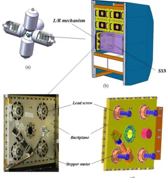
As one of scientific exploration oriented carriers, the Chi-nese Space Station Microgravity Platform (SSMP) provides a higher level of controllable environment for samples and instruments and facilitates delicate manipulations in diverse new technology experiments, such as material sciences, mi-crogravity fluid physics and biotechnology (Xie et al., 2016; Wang et al., 2014; Liu et al., 2006). The L/R mechanism is configured in parallel, developed and equipped supportively for the SSMP, and its hierarchical relation is illustrated in Fig. 1. The conceptual model of the Chinese Space Station, consists of a core chamber module and four experimental chamber modules. In each experimental module, each
sci-entific research experiment rack is fixed in parallel with the others (Zhou, 2013; Liu et al., 2014). Two auto L/R mech-anisms are assembled into both sides of each scientific re-search experiment rack to lock the SSMP. During the shuttle launching stage, the SSMP is securely locked by eight lead screws of the L/R mechanisms on both sides. While arriving at the scheduled orbit of the space station, the lead screws on each side are driven inversely to release the SSMP for micro-gravity experiments.
in-Figure 1.Hierarchical relation(a)conceptual model of the Chinese Space Station;(b)scientific research experimental rack and the SSMP with two L/R mechanisms in a locked status;(c)physical prototype and(d)3-D model of the L/R mechanism on a side of the SSMP.
creasing global competition. Tolerance assignments for me-chanical parts and assembly of a product play an important role in the accuracy performance of the product, since it is closely connected with components’ tolerance (Merlet, 2006; Hao and Kong, 2016; Hao and Merlet, 2005; Huang et al., 2016; Huang and Kong, 2010; Li et al., 2016). As one of the crucial tasks in a product life cycle, tolerance synthesis for mechanical parts and assembly of a product, which is gener-ally regarded as tolerance design, is a typical iterative proce-dure. It ranges from tolerance initialization to final reason-able tolerance determination, in which constraints such as manufacturing capability, performance quality and produc-tion cost are considered (Moroni and Polini, 2003; Pasupathy et al., 2003). There are two problems to be addressed: (a) how the mechanism tolerance is assigned, so that manufacturing complexity is reduced without much loss in quality (Singh et al., 2009a; Chen and Ji, 2005; Chlebus and Wojciechowska, 2016; Jeang, 2001; Lyu et al., 2006; Rout and Mittal, 2006, 2007, 2008; Li et al., 2015); and (b) how the synthesis
ap-proach is devised so that process data can be promoted in precision and efficiency (Singh et al., 2009b; Huang, 2013).
1.1 Mechanism tolerance synthesis review
coor-dination of wing’s swing and pitch. Yin et al. (2018) inves-tigated tolerance design for spatial mechanisms with the use of both the extremum and the probability methods. In com-parison with several surrogate models, the tolerance was op-timized and thus manufacturing cost is significantly reduced. DOE based tolerance design has drawn close attention in recent years for engineering applications. Employing the concept of Taguchi S/N ratio, Rout and Mittal (2006, 2007, 2008) utilized the inner and outer orthogonal array to iden-tify significant parameters of a 2-DOF planar manipulator with two revolute joints for optimum tolerance. Optimum tolerance of the manipulator with payload was finally allo-cated, and was validated by Monte Carlo (MC) simulation. Huang (2015) developed a Taguchi based optimum tolerance design for a function generation mechanism with joint clear-ance, where the total cost of assembly was minimized while satisfying the accuracy requirements. Insight on parameter variances of this mechanism was provided with the sensitive maps, and the efficiency and practicality were demonstrated with the proposed method. Li et al. (2015) investigated the tolerance design problem of a 6-DOF space docking mecha-nism using uniform design, and concerned the efficiency and precision of MC simulation in DOE. The tolerance of the component in the mechanism was properly broadened with-out any loss of with-output accuracy, and the manufacturing cost was reduced to a certain extent. Huang (2004, 2013), Huang and Kong (2010) and Zhou (2001) made a comprehensive introduction to the advantages of number-theoretic method (NTM), and exhibited the significant precision and surpris-ing efficiency of NTM in tolerance design and process sim-ulation, which made the comprehensive theory of NTM start to serve the manufacturing in engineering.
1.2 DOE based tolerance synthesis methodology In a process for mechanism manufacturing, the capacity is constantly influenced by multiple stochastic factors, and presents fluctuant. The tolerance assigned may not be pos-sibly dynamically suitable in practice. Therefore, tolerance assignment should be with the characteristics of redundancy and flexibility. Tolerance synthesis approach should have high analytical precision and efficiency, and generate toler-ance assignments with completeness and representativeness, that could be actively resistant to potential failure, due to in-stability of manufacturing capability.
NTM offers a possible solution for this problem. The essence of NTM is to determine a point-set in a s -dimensioned super-cube, where the points in the set are uni-formly distributed (Fang and Wang, 1994). Till now mathe-maticians have proposed several types of set such as Hua– Wang set (Hua and Wang, 1972), Halton set (Halton, 1960; Chi et al., 2005), Niederreiter set (Niederreiter, 1992) and Sobol set (Sobol, 1967; Bratley and Fox, 1988). They are all termed as low discrepancy sequence (LDS). The initial tar-get of LDS aims at improving MC simulation performances,
which are prevailing over the traditional pseudo-random set, then the LDS is introduced in the field of DOE, and as the ba-sis, uniform DOE is established (Fang and Wang, 1994) with GLP-set (Hua and Wang, 1972). Uniform DOE pays more attention on distributional uniformity other than symmetri-cal comparability of experiment points. It could disclose sys-tem information with the fewest representative points. On the contrary, the experiment points construct an optimum and uniform coverage of experiment space.
With this advantage, the uniform DOE array, composed of different levels of tolerance in a mechanism, could con-struct plenty of candidate tolerance assignments. They are optimally and uniformly distributed within the experiment space. As manufacturing capability fluctuates, these assign-ments can be valuable and robustly adapt to variation of man-ufacturing capability.
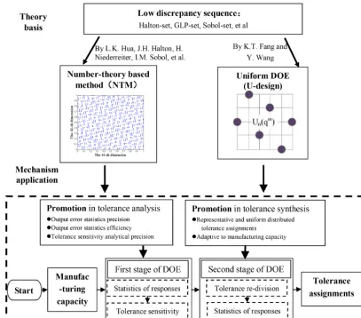
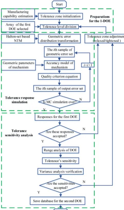
In this paper, the accuracy model for the L/R mechanism is established firstly. For a precise and efficient simulation process, the Halton-set based MC simulation, is introduced in tolerance analysis of the L/R mechanism. Then, tolerance synthesis is proposed consisting of two stages. The first stage of DOE, provides tolerance sensitivity, and the second one, applies uniform DOE to generate tolerance assignments with representativeness and uniformity, against capacity instabil-ity and manufacturing complexinstabil-ity. The flowchart of the tol-erance synthesis applying both NTM and uniform DOE is illustrated in Fig. 2.
Building on the above advances, this paper focuses on tol-erance analysis and synthesis towards application in the L/R mechanism. The reminder of this article is organized as fol-lows: Sect. 2 briefly introduces the structure and principle of the L/R mechanism; Sect. 3 completes accuracy modeling for the L/R mechanism, and conducts tolerance analysis with Halton-set based MC simulation; Sect. 4 details the tolerance synthesis procedures for the L/R mechanism and illustrates the practicability for a case study; Conclusions are drawn in Sect. 5.
2 L/R mechanism description
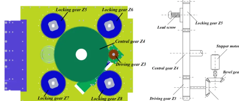
The architecture of a L/R mechanism is illustrated in Fig. 3. The stepper motor on the backside, drives the bevel gear Z1, then revolve gears Z2 and Z3 that are connected together. Driven by a central gear Z4, four branches of gears rotate simultaneously, making four lead screws move forward as synchronous as possible for the locking gears Z5, Z6, Z7, and Z8. The SSMP is securely locked by contacting the ends of the four lead screws, with the slots on both sides of the SSMP. While arriving at scheduled orbit, four lead screws on each side are then driven inversely to release the SSMP.
Figure 2.Flowchart of tolerance synthesis with both NTM and uniform DOE.
raise impact damage structurally by harmonic response of the SSMP’s vibration during the launch stage; Secondly, the unbalanced locking supports on the SSMP inversely make lead screws unable to form symmetric or regular deforma-tion, which also poses a potential threat to the shuttle struc-turally. However, higher manufacturing accuracy for the L/R mechanism would inevitably increase manufacturing com-plexity; it may be unreachable to manufacturing capability. Therefore, an optimum compromise between tolerance and capacity for the mechanism is essential to vouch the system’s high reliability and security.
3 Modelling and simulation
Geometrical errors of the L/R mechanism come from the un-certainty of connected components’ position and orientation during the manufacturing stages, and complicate the influ-ence of the output errors, which are represented by the end errors of the lead screws. In this section, an accuracy model of the L/R mechanism using vector differential algorithms is established, which provides linear relations between
geomet-rical errors and output errors. On improving accuracy simu-lation precision and efficiency, the Halton-set based MC sim-ulation is introduced and compared to the traditional pseudo-random set based MC simulation.
3.1 Mechanism accuracy modeling
Both the L/R mechanisms are symmetrically configured on both sides of the SSMP as shown in Fig. 1. Each side can provide enough geometric information for accuracy analysis. Four lead screws are fixed on the backplane of the L/R mech-anism, and they are guided by a gear train to synchronously travel forward until their ends contact slots of the SSMP on a side.
The imperfectness of assembly generates locational errors δxp,δyp,δzp,δα,δβandδγof the backplane, they are with respect to the nominal position of the scientific research ex-periment rack; similarly, each lead screw on the backplane has locational errors δai,x, δai,y, δai,z, and angular errors
Figure 3.Configuration of transmission train of the L/R mechanism.
errors from the engaged gears and assembly error. However, repetitive experiments had indicated the axial error of lead screw assembled weighted majority among the translation er-rors, therefore, the transmission errors are not included in the mechanism accuracy model. The output errors δbi,x, δbi,y andδbi,z refer to inaccuracy between the end of each lead screw and nominal contact center on a side of the SSMP.
Frames{OB}and{OA0}attaching at the nominal centers on a surface of the SSMP and mechanism’s backplane, are outlined in Fig. 4 respectively. Frame{OA0}has a positional error vectorδp(δxp,δyp,δzp)T and an angular error vector
δ(δα,δβ,δγ)T with respect to the base frame{OB}. Four lead screws in both coordinate frames form four closed kine-matic loops. Since all the lead screws are centrosymmetric about the z0axis of coordinate frame{OA0}, either closed-loop kinematic chain is established independently and repre-sentatively.
In Fig. 4, the closed-loop kinematic chainOB−OA0−A0 i−
Bi0can be expressed with a vector equation as
bi =p+R(ai+liui) (i=1,2,3 or 4) (1) whereRrefers to the rotational matrix of frame{OA0}with nominal orientation anglesα,βandγ, aboutx,yandzaxes, and can be written as
R=
cosγ −sinγ 0 sinγ cosγ 0
0 0 1
cosβ 0 sinβ
0 1 0
−sinβ 0 cosβ
1 0 0
0 cosα −sinα 0 sinα cosα
Differentiating both sides of Eq. (1) yields
δbi =δp+δR(ai+li·ui)+R(δai+δli·ui+li·δui) (2)
whereδbi (δbi,x,δbi,y,δbi,z) denotes the end error vector of theith lead screw in frame{OB};δp(δxp,δyp,δzp)T refers to the positional error vector of the backplane with respect to base frame{OB};δRdenotes perturbation of the rotational matrixRof frame{OA0}with regard to the base frame{OB}; ui(ux,uy,uz)T refers to the unit vector of theith lead screw;
δuirepresents a deviation ofui, and can be expressed as
δui=1uiui=
0 −δuz δuy
δuz 0 −δux
−δuy δux 0 ux uy uz (3)
where1uidenotes the antisymmetric tensor ofδui.
δRin Eq. (2), has to deal with the perturbation vectorδ (δx,δy,δz)T of the nominal anglesα,β, andγ, with respect to base frame{OB}. Therefore,δcan be detailed as δ=δγ 0 0 1 +δβ
cosγ −sinγ 0 sinγ cosγ 0
0 0 1
0 1 0 +δα
" cosγ −sinγ 0 sinγ cosγ 0
0 0 1
# " cosβ 0 sinβ 0 1 0
−sinβ 0 cosβ
# " 1 0 0 # δ= δx δy δz =
−sinγ δβ+cosγcosβδα cosγ δβ+sinγcosβδα
−sinβδα+δγ
The antisymmetric tensor ofδcan be denoted as
1R=
0 −δz δy
δz 0 −δx
−δy δx 0
Figure 4.Assembled L/R mechanism with the SSMP and kinematic diagram for this simplified L/R mechanism.
Therefore, the matrixδRin Eq. (2) can be written as
δR=1RR=
0
−sinβδα+δγ
−cosγ δβ−sinγcosβδα
sinβδα−δγ 0
−sinγ δβ+cosγcosβδα
cosγ δβ+sinγcosβδα sinγ δβ−cosγcosβδα
0
R
Since the nominal orientation anglesα,β, andγof the frame
{OA0}with respect to base frame{OB}are all zeros in the ge-ometric configuration of the SSMP and the L/R mechanism, δRcan be simplified as
δR=1RR=
0 −δγ δβ
δγ 0 −δα
−δβ δα 0
R (4)
where1Ris an antisymmetric tensor ofδ; letci =R(ai+
liui), Eq. (2) can be rewritten in a compact form as
δbi = E 1Tci
δp
δ
+R· δai+δli·ui+li·1ui·ui
(5)
whereEis a 3×3 unit matrix;1ciis an antisymmetric tensor
of vectorci.
The nominal parameters in Eq. (5) can be determined as follows: the nominal orientation anglesα,β, andγ of the backplane are set zeros, therefore the orientation matrix R
becomes a 3×3 unit matrix; The unit vectorui with nomi-nal value (0,0,−1)T for each lead screw synchronizes with frame{OA0}while micro rotating of frame{OA0}occurs. The
xandycomponents of vectorδuican be approximated with micro rotational angles,1θ1and1θ2, for a lead screw about its ownx andy axes, respectively, andzcomponent ofui is zero. Thus, Eq. (5) can be unfolded as follows
δbi,x δbi,y δbi,z =
1 0 0 0 ai,z−li −ai,y 0 1 0 li−ai,z 0 ai,x 0 0 1 ai,y −ai,x 0
δxp
δyp
δzp δα δβ δγ + δai,x δai,y δai,z + 0 0
−δli
+li
0 −δui,z δui,y
δui,z 0 −δui,x
−δui,y δui,x 0 0 0 −1 (6)
whereδli refers to the axial error1li of theith lead screw which is contributed by the gear train in the L/R mechanism, and is irrelevant with other geometrical errors investigated above.
3.2 Halton-set based MC simulation
im-Table 1.Nominal parameters for the L/R mechanism.
Nominal locations of lead screws Nominal contacts points of lead screws
ai,x(mm) ai,y(mm) ai,z(mm) bi,x(mm) bi,y(mm) bi,z(mm)
1 150 150 0 150 150 0
2 −150 150 0 −150 150 0
3 −150 −150 0 −150 −150 0
4 150 −150 0 150 −150 0
Table 2.Geometric errors of the L/R mechanism.
1xp(mm) 1yp(mm) 1zp(mm) 1α(◦) 1β(◦) 1γ(◦) 1ai,x/1ai,y(mm) 1ai,z(mm) 1θ1/1θ2(◦) 1l(mm)
±0.3 ±0.3 ±0.4 ±0.3 ±0.2 ±0.3 ±0.25 ±0.3 ±0.12 ±0.1
proving the precision and efficiency for a MC simulation is essential.
In recent decades, the NTM gradually became popular in computational mathematics area, and prevailed over tradi-tional MC techniques in precision and efficiency. Instead of pseudo-random set in statistical simulation, the NTM applies LDS, whose points scatter evenly in a unit cubic, and whose regularity can be evaluated mathematically. The NTM based simulation could provide a higher convergence rate induced by its computation complexity of O(logsN/N) than that in-duced by the one ofO(N−1/2) provided by pseudo-random based MC simulation, wheres represents the dimension of the investigated problem.
For Halton sequence (Halton, 1960), each pointkcan be represented by am-ary expansion:
k=b0+b1m+b2m2+. . .+brmr (7) wheremis a prime number less than integerbi,0< bi< m− 1,i=0,1,2. . .r. The component of each point in Halton-set can be represented by a radical inverse functionym(·) defined as
ym(k)=b0m−1+b1m−2+. . .+brm−r−1 (8) whereym(k)∈(0,1), and the each point,Xk, in Halton-set withs-dimension, can be expressed as
Xk=ym1(k), ym2(k), . . ., yms(k)
(9)
where a set of pairwise coprimem1,m2, . . ., ms are selected as dimensional bases. Generally, the first s prime numbers are favorable in simulation.
3.3 Effectiveness comparison
A comparison to output errors of the L/R mechanism for tra-ditional (pseudo-random based) and Halton-set based MC simulation, are performed. All the parameters for the L/R mechanism are listed in Table 1. All the geometric errors
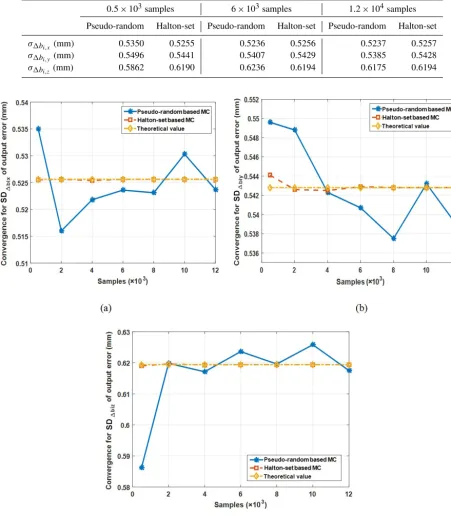
in Eq. (6) are presumed to conform to uniform distribution within their tolerance zone, and listed in Table 2. The sim-ulation comparison employs the sample size of 0.5×10³, 2.0×10³, 4.0×10³, 6.0×10³, 8.0×10³, 1.0×10⁴, and 1.2×10⁵. Standard deviations of output errors are repre-sented by thex,y andzerror of the end of each lead screw and listed in Table 3. Variations of standard deviation con-vergences are shown in Fig. 5.
The relative errorσRis selected to evaluate the precision between two approaches and defined as
σR=
|σS−σT|
σT
×100 % (10)
whereσSrepresents standard deviation simulated with either approach, andσTis theoretical standard deviation with ana-lytic error model in Eq. (6).
Figure 5 illustrates that the standard deviation σ1bi,x,
σ1bi,y, orσ1bi,z of the L/R mechanism’ output errors with
Halton-set based MC simulation, has a higher convergence rate than those with pseudo-random based one. The theoret-ical values of the statisticsσ1bi,x,σ1bi,y, orσ1bi,z, are
pro-cessed with the L/R mechanism error model in Eq. (6), and based on the nominal parameters in Table 1 and parameters’ errors in Table 2. To reach the same simulation precision, for instance, we simply define a relative error ofσR≤0.1 %. For
σ1bi,x, it is achieved with a sample size of 500 by
Halton-set. It is smaller than that of 1.2×10⁵ by pseudo-random based MC simulation; forσ1bi,y, it is achieved with a sample
size of 2×10³ by Halton-set, and it is smaller than that of 4×10³by pseudo-random based MC simulation; forσ1bi,z,
it is achieved with a sample size of 500 by Halton-set, and it is also smaller than that of 2×10³by pseudo-random based MC simulation. Additionally, the convergences forσ1bi,y and
σ1bi,z with pseudo-random based MC simulation fluctuate
Table 3.Standard deviationsσof the L/R mechanism output error with pseudo-random and Halton-set based MC simulation.
0.5×10³samples 6×10³samples 1.2×10⁴samples
Pseudo-random Halton-set Pseudo-random Halton-set Pseudo-random Halton-set
σ1bi,x (mm) 0.5350 0.5255 0.5236 0.5256 0.5237 0.5257 σ1bi,y (mm) 0.5496 0.5441 0.5407 0.5429 0.5385 0.5428 σ1bi,z(mm) 0.5862 0.6190 0.6236 0.6194 0.6175 0.6194
Figure 5.Convergence contrasts with pseudo-random and Halton-set based MC simulation for standard deviation of output errors for the L/R mechanism.
We have found that as the dimension of a problem in-creases, the priorities in analytical precision and efficiency based on NTM are more significant over traditional Monte Carlo simulation. This simulation belongs to a 12-dimension problem, and Li et al had applied Sobol-set based MC in
in the construction methods of different point sets. With the deepening of the number theory research, point set construc-tion methods to improve the accuracy and efficiency of anal-ysis will continue to emerge.
4 Tolerance synthesis
Taguchi (Rout and Mittal, 2006, 2007, 2008) suggests that the quality of a product is not ensured in the checking stage, but determined in the design stage. A reasonable tolerance assignment could not only facilitate production process but also bring about better performance of a product.
Generally, traditional tolerance synthesis for a mechanism is considered as a typical optimization technique. It aims at achieving a compromise between tolerance and cost, under constraints of various quality criterions. The optimized toler-ance is then directly applied in the mechanism manufactur-ing, without much modification. This is currently a general process for mechanism development in a laboratory.
However, in contemporary manufacturing enterprise, there are plenty of stochastic factors disturbing process capacity dynamically; traditional synthesis approach is not perfectly suitable to modern production. It is necessary to propose an enterprise oriented mechanism’s tolerance synthesis ap-proach, which generates tolerance assignments with enough flexibility to adapt to stochastic variations of capacity.
4.1 DOE based synthesis methodology
In view of DOE, different tolerance as factors in a mecha-nism can be considered as independent dimensions. They are spanning a multi-dimensioned space, which can be regarded as “tolerance space”. In this space, the boundaries can be es-timated by manufacturing capability, potentially feasible tol-erance assignments are enveloped.
In tolerance space, different tolerance has their corre-sponding sensitivities to mechanism output performance. Tolerance sensitivity can be provided through range analysis. Then we can use their sensitivities to update levels of differ-ent tolerance, as level variation of any tolerance contributes equivalent influence on the mechanism output performance.
With the newly updated levels, how they can be merged into expected tolerance assignments, is an interesting and practical problem. An intuitive idea is to enumerate all the levels of all the factors, however, as the number of tolerance factor or levels increases, the sorting process may possibly result in a combinational explosion.
A compromise approach is to select representative combi-nations of levels in tolerance space. The representative com-binations, as tolerance assignments, can be determined by a uniform DOE array, with good uniformity and neat compa-rability. They can optimally cover the tolerance space and be tolerant to capacity variation well.
The uniform DOE, short for uniform design, is proposed in the 1980s by Fang and Wang (1994), and is distinct from
typical orthogonal design and Latin square design. The uni-form experiment points are uniuni-formly scattered within the whole experiment space, and fewest representative experi-ment points can disclose most information of a system, other than the rest types of DOE.
Uniform DOE (Fang and Lin, 2007) is particularly profi-cient in tackling high dimensional problem with factors and levels of large numbers. Uniformity of a uniform DOE can be measured through L2-discrepency as follows:
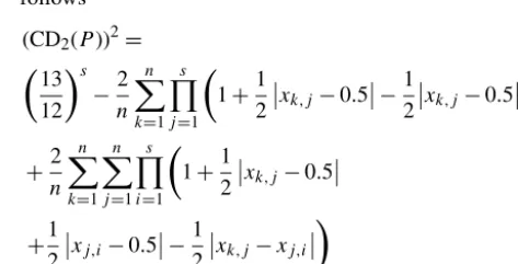
Given a s-dimensioned super-cube Cs= [0,1]s, a set of experiment pointsP = {x1, . . ., xn} is constructed and dis-tributed within the entire experiment space as uniformly as possible.L2-discrepency, short for CD2(·), is used to evalu-ate the uniformity of the point setP and can be written as follows
(CD2(P))2= 13 12 s −2 n n X
k=1 s Y
j=1
1+1
2
xk,j−0.5 −
1 2
xk,j−0.5 2 +2 n n X
k=1 n X
j=1 s Y
i=1
1+1
2
xk,j−0.5
+1
2
xj,i−0.5 −
1 2
xk,j−xj,i
(11)
where xk=(xk,1, . . ., xk,s) is the kth experiment point. In terms of the point set generation rule, the experiment space is consistently filled with uniform points of different quan-tity, therefore, the set of tolerance assignments, as experiment points, can be ultimately formulated. With a proper uniform design array, a tolerance assignment set can also be available.
4.2 DOE based synthesis procedure
In the first stage of DOE, a proper DOE array is firstly se-lected in terms of the tolerance factor. Tolerance levels are initially evenly divided with geometric tolerance determined by manufacturing capacity, since we do not have any knowl-edge of their sensitivity. Then Halton-set based MC simula-tion is employed for DOE response, please refer to Sect. 3.2. Through range and variation analysis techniques, the sensi-tivities of geometric tolerances are subsequently obtained. Figure 6 detailed the scheme of the first stage of DOE for factor sensitivities, which mainly includes preparations for 1-DOE, tolerance response simulation and tolerance sensi-tivity analysis.
Figure 6.Scheme for the first stage of DOE for the L/R mecha-nism’s tolerance synthesis.
4.3 Definition and Strategy
DOE based tolerance synthesis for a mechanism has to: de-fine response function, arrange tolerance factors and levels, and devise other detail strategies related to tolerance assign-ment. They are addressed as follows.
4.3.1 Response function definition
The tolerance stack-up is used to reflect the success rate of the assembled mechanism, and evaluate manufacturing qual-ity whether this tolerance assignment is acceptable. It in-volves two aspects: radical error1ri of each lead screw and non-synchronous error1zof all 4 lead screws of the
mecha-nism, they can be respectively defined as
1ri = q
1x2p,i+1yp,i2 ≤1r0 (12)
1z=max(1zp,i−1zp,j)≤1z0
(i, j=1,2,3 or 4) (i6=j) (13) where1xp,iand1yp,idenote the end errors of a lead screw alongx andy axis respectively, and can be obtained from Eq. (6).1r0represents the allowed threshold of a radical er-ror in a side surface of SSMP in Fig. 4.1z0is the permitted threshold of non-synchronous error.
It is noted that there is a statistical process. We define an event “Mi” as an occurrence of the radical error1ri of the
ith screw’s end, within the threshold of1r0, which can be ex-pressed as1ri< 1r0. Then another event “N” is defined as an occurrence of non-synchronous error alongzaxis among the ends of screws, within a threshold of 1z0, which can be expressed as “1z < 1z0”. The tolerance stack-up is the probability of all the events “Mi” (i=1, 2, 3, or 4) and “N”, occurring at the same time. Thus, the tolerance stack-up can be expressed as a probability of multi-event production, since they are independent with each other:
P(M1M2M3M4N)=P(N|M1M2M3M4N)
×P(M1|M2M3M4)×P(M2|M3M4)
×P(M3|M4)×P(M4)
(14)
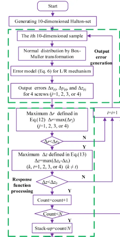
We can take 99.73 % as a threshold of the tolerance stack-up, in terms of “6σ” principle in production quality control the-ory. It means if a combination of tolerance levels in the uni-form DOE yields a responseP(M1M2M3M4N)>99.73 %. This combination can be accepted as one of potentially feasi-ble candidate tolerance assignment. A detailed schematic for simulation process is outlined in Fig. 7.
4.3.2 Arrangements for factors and levels
In a tolerance synthesis, geometric tolerance of a mechanism as factors are considered before a proper DOE array is deter-mined. The first stage of DOE is designed to obtain a general knowledge of sensitivity of different tolerance factor. There-fore, over-condensed levels are not necessary for DOE ana-lytical efficiency.
4.3.3 Strategy for level re-division
For the second DOE stage, interval between adjacent lev-els of a tolerance factor follows inverse proportion to its own sensitivity, as to place an equivalent impact on mecha-nism output performance. The level re-division follows three steps:
levels of the rest factors is expressed as:
1i =
Ri
R ×
Thi−Tli
n (15)
whereRidenotes the sensitivity of theith tolerance fac-tor; Thi and Tli denote the upper and lower bounds of theith tolerance factor, respectively,ndenotes the ex-pected number of levels.
b. Determining new levels of all factors as:
Li,j=Tli+1i×(j−1)
0< j <
Th i−Tli
1i
(16)
whereLi,j refers to thejth level of theith factor, andj is an integral number.
c. Simulating with Halton-set based MC approach with these newly updated levels, and yielding tolerance stack-ups as responses.
4.4 Illustrative example
The L/R mechanism discussed is shown in Fig. 4, the whole tolerance synthesis is presented as follows:
4.4.1 Parameters initialization Quality index requirement
The radical error1r0defined in Eq. (12) is set with 1.6 mm, which means radical deviations for all the screw ends are re-stricted within 1.6 mm. The non-synchronous error1z0 de-fined in Eq. (13) is configured with 1.6 mm. To ensure the manufacturing quality, the tolerance stack-up should be no less than 99.73 % in terms of “6σ” principle.
Traditional tolerance synthesis approach comes from ex-perience in practice, does not place sufficient concern on the sensitivity of different tolerance. That makes the toler-ance assignment become less flexible, and limits the assem-bly application. In terms of experience, the tolerance assign-ment is obtained and listed in Table 4, and whose stack-up is processed with the scheme described in Fig. 7, and finally reaches up to 99.99 % (>99.73 % of “6σ”). This tolerance assignment is acceptable for a successful assembly of the L/R mechanism, however, as manufacturing capacity varies, its feasibility is still doubtful.
Tolerance factors’ initialization
All the geometric tolerance factors are initialized as follows: the permitted limitations of dimensional tolerances involv-ing1xp,1yp,1zp,1ai,x,1ai,y,1ai,z,1lare no less than
±0.1 mm; and permitted those of angular tolerances involv-ing 1α,1β,1γ,1θ1,1θ2are no less than ±0.1◦. Since the technological process tolerance 1ai,x for a lead screw,
Figure 7.Scheme of Halton-set based simulation for the tolerance stack-up and for each column in the uniform DOE array.
resembles that of1ai,y, they are regarded as the same fac-tor; similarly, the same analysis is for1θ1 and1θ2 which can also be regarded as the same factor. Therefore, 10 tol-erance factors are finally determined:1xp,1yp,1zp,1α,
1β,1γ,1ai,x(or1ai,y),1ai,z,1θ1(or1θ2) and1l.
4.4.2 The first stage of DOE
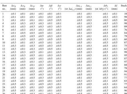
With DOE based tolerance synthesis discussed above, the or-thogonal arrayL27(310) is chosen for the first stage of DOE. It accommodates 10 factors, three levels for per factor and 27 combinations, can be considered as an appropriate arrange-ment for compromise between efficient and precise simula-tion, and is listed in Table 5.
Table 4.Experience based tolerance assignment for the L/R mechanism.
1xp 1yp 1zp 1α 1β 1γ 1ai,x 1ai,z 1θ1 1l Stack-up (mm) (mm) (mm) (◦) (◦) (◦) (or1ai,y) (mm) (or1θ2) (mm) (%)
(mm) (◦)
±0.2 ±0.2 ±0.2 ±0.15 ±0.15 ±0.15 ±0.2 ±0.2 ±0.15 ±0.2 99.99
Table 5.Levels division ofL27(310) array for geometric tolerance factors.
1xp 1yp 1zp 1α 1β 1γ 1ai,x 1ai,z 1θ1 1l
(mm) (mm) (mm) (◦) (◦) (◦) (or1ai,y) (mm) (or1θ2) (mm)
(mm) (◦)
Level 1 ±0.1 ±0.1 ±0.1 ±0.1 ±0.1 ±0.1 ±0.1 ±0.1 ±0.1 ±0.1 Level 2 ±0.3 ±0.3 ±0.3 ±0.3 ±0.3 ±0.3 ±0.3 ±0.3 ±0.3 ±0.3 Level 3 ±0.5 ±0.5 ±0.5 ±0.5 ±0.5 ±0.5 ±0.5 ±0.5 ±0.5 ±0.5
Table 6.L27(310) orthogonal array for responses with a sample size of 105using Halton-set based MC simulation.
Run 1xp 1yp 1zp 1α 1β 1γ 1ai,x 1ai,z 1θ1 1l Stack-up no. (mm) (mm) (mm) (◦) (◦) (◦) (or1ai,y) (mm) (mm) (or1θ2) (◦) (mm) (%)
1 ±0.1 ±0.1 ±0.1 ±0.1 ±0.1 ±0.1 ±0.1 ±0.1 ±0.1 ±0.1 100.0 2 ±0.1 ±0.1 ±0.1 ±0.1 ±0.3 ±0.3 ±0.3 ±0.3 ±0.3 ±0.3 98.68 3 ±0.1 ±0.1 ±0.1 ±0.1 ±0.5 ±0.5 ±0.5 ±0.5 ±0.5 ±0.5 80.26 4 ±0.1 ±0.3 ±0.3 ±0.3 ±0.1 ±0.1 ±0.1 ±0.3 ±0.3 ±0.3 98.70 5 ±0.1 ±0.3 ±0.3 ±0.3 ±0.3 ±0.3 ±0.3 ±0.5 ±0.5 ±0.5 89.55
6 ±0.1 ±0.3 ±0.3 ±0.3 ±0.5 ±0.5 ±0.5 ±0.1 ±0.1 ±0.1 76.79
Table 7.Variance analysis for the sensitivities of the tolerance factors.
Source of variation SS (Sum of squares) Degrees of freedom Mean square F0
Factor 1:1xp 1.505×10⁻⁴ 2 – –
Factor 2:1yp 1.839×10⁻⁴ 2 – –
Factor 3:1zp 2.812×10⁻⁵ 2 – –
Factor 4:1α 0.1676 2 8.38×10⁻² 183.62∗
Factor 5:1β 0.1690 2 8.45×10⁻² 185.18∗
Factor 6:1γ 0.0051 2 2.6×10⁻³ 5.63∗
Factor 7:1ai,x(or1ai,y) 13.022×10⁻⁵ 2 – –
Factor 8:1ai,z 0.0015 2 – –
Factor 9:1θ1(or1θ2) 3.28×10⁻⁴ 2 – –
Factor 10:1l 0.0016 2 – –
SS1e (factor 1–3 and 7–9) 0.0091 20 4.56×10⁻⁴ –
SST 0.3509 26 – –
∗Significant at 0.025 % (F
0.025(2,12)=5.1).
For precise tolerance sensitivity in the first stage, a conver-gence comparison with pseudo-random and Halton-set based MC simulation is conducted according to the schemes shown in Figs. 6 and 7. Sample sizes are 1×10⁴, 2×10⁴, 4×10⁴, 6×10⁴, 8×10⁴and 1×10⁵. The convergences of sensitivities for 10 tolerance factors are plotted in Fig. 8.
From the convergence of sensitivities for 10 tolerance fac-tors, obtained in Fig. 8, we can be found that the tolerance sensitivities convergence with Halton-set based MC simula-tion, generally maintains a steadier process than that with pseudo-random based one. By comparison, these statistics with Halton-set based NTM simulation is more reliable than that with pseudo-random in convergence precision. The final tolerance sensitivities, with a sample size of 105 Halton-set based MC simulation is depicted in Fig. 9. The analysis of variance is then carried out, to verify the tolerance sensitivi-ties as listed in Table 7.
Tolerance factor sensitivities have been yielded through range analysis in Fig. 9. Variance analysis in Table 7 confirms that the orientation angular errors,1αand1β, for backplane of the L/R mechanism are the most sensitive factors, and they should be tightly controlled during the manufacturing pro-cess. Therefore, in the second stage of DOE for tolerance assignment, the sensitive factors,1αand1β, are configured with top levels ±0.1◦ of permitted tolerances; the insensi-tive ones such as1xp,1yp,1zp, and1ai,x(or1ai,y), can be assigned with a more relaxed tolerance±0.5 mm; and the rest ones including 1γ,1ai,z,1θ1 (or 1θ2) and 1l with their permitted tolerance zones, are put into the second stage of the uniform DOE for final tolerance assignment.
4.4.3 The Second stage of DOE
As discussed in Sect. 4.2, the more/less sensitive a factor is, the narrower/broader an interval of adjacent levels should be in general. Therefore, the interval for levels is expected to
Figure 9.Tolerance stack-up sensitivities for the tolerance factors.
be inversely proportional to their sensitivities. The uniform array of U20(44) is properly enough by accommodating to 4 factors, 4 levels per factor and 20 combinations of levels. The combinations of different levels among factors with distribu-tional regularity and uniformity, have an optimum coverage of the tolerance space, and avoid enumeration that may pos-sibly result in a combination explosion. The levels re-divided for factors1γ,1ai,z,1θ1(or1θ2) and1lare contained in Tables 8 and 9.
4.4.4 Tolerance assignment and evaluation
Table 8.Tolerance factor levels re-division for U20(44) array within tolerance zones (part A).
Factor 6 Factor 8 Factor 9 Factor 10 Level no. (1γ) (mm) (1az) (mm) (1θ1(or1θ2) (◦) (1l) (mm)
Level 1 ±0.10 ±0.10 ±0.10 ±0.10
Level 2 ±0.14 ±0.16 ±0.23 ±0.16
Level 3 ±0.17 ±0.22 ±0.37 ±0.22
Level 4 ±0.21 ±0.28 ±0.50 ±0.27
Table 9.Tolerance factor levels re-division for U20(44) array within tolerance zones (part B).
Factor 6 Factor 8 Factor 9 Factor 10 Level no. (1γ) (mm) (1ai,z) (mm) (1θ1(or1θ2) (◦) (1l) (mm)
Level 1 ±0.30 ±0.30 ±0.10 ±0.30 Level 2 ±0.34 ±0.36 ±0.23 ±0.36 Level 3 ±0.37 ±0.42 ±0.37 ±0.42 Level 4 ±0.41 ±0.48 ±0.50 ±0.47
Halton-set based MC simulation, are produced in Tables 10 and 11.
Generally, the complexity of product manufacturing can be lowered down, as the tolerance is properly amplified. There may still be reachable compromise between reliabil-ity and economy in tolerance assignments. We usually define different functions to evaluate manufacturing consumption. Typical cost-tolerance functions, such as linear, exponential, inverse square, and power series one (Singh, 2009a, b), could precisely express the relations between tolerance and con-sumption. When applied in a particularly compound process, these types of cost-tolerance functions need to be modified with experience.
Compared to tolerance determined by experience in tol-erance relaxation, we simply choose the linear accumula-tive tolerance as cost-tolerance function, to make comparison of tolerance relaxation. Thus, the cost-tolerance dimensional and angular functions,TP
d andT
P
a, can be defined as
T6d=1xp+1yp+1zp
+4(1ai,x+1ai,y+1ai,z)+41l
T6a=1α+1β+1γ+4(1θ1+1θ2) (17)
Relaxation of dimensional and angular tolerance, ATd and
ATa, can be evaluated as
ATd=
T62d−T61d
T61d
×100 %
ATa=
T62a−T61a
T61a
×100 % (18)
where TP
1d andT
P
1a denote the dimensional and angular
accumulated tolerance, respectively. They are originally de-termined by experience in terms of Table 4, with TP
1d=
3.8 mm and TP
1a=1.65
◦.TP
2d and T
P
2a of each
assign-ment in rows in Tables 10 and 11 are processed with Eq. (14), and their relaxation (ATdandATa) are finally tabulated.
4.5 Discussion
Tolerance assignments in Tables 10 and 11 in series with uni-form DOE, provide potentially feasible candidates with the application for the L/R mechanism manufacturing. All the stack-ups of assignments as response, are upper than 99.73 % in terms of “6σ” principle. It indicates that all of them satisfy manufacturing quality criteria. However, this does not mean all the initial tolerance bounds restricted by capacity, can def-initely generate satisfying stack ups, since there may still be a few assignments unfeasible, however, it will not disable tol-erance synthesis.
The relaxation,ATd andATa, of the tolerance assignments
with positive signs, indicate the tolerance of the assignment is relaxed, compared to that of experience based tolerance assignment. Those with negative sign, indicate assignments a contractive tolerance. However, the majority of the mech-anism’s tolerances are significantly relaxed considering:ATd
is up to 144.7 % of the combination 9 in Table 11, andATa
is up to 179.4 % of the combination 19 in Table 11; even though there are seven combinations with negative relaxation ofATa. Tolerance assignments with positive amplifications of
ATd andATa as candidates can facilitate the manufacturing
process of the L/R mechanism.
mecha-Table 10.Array U20(44) for responses with a sample size of 105using Halton-set based MC simulation (part A).
1xp 1yp 1zp 1α 1β 1γ 1ai,x 1ai,z 1θ1 1l Stack-up ATd ATa
(mm) (mm) (mm) (◦) (◦) (◦) (or1ai,y) (mm) (or1θ2) (mm) (%) (%) (%)
(mm) (◦)
1 ±0.5 ±0.5 ±0.5 ±0.1 ±0.1 ±0.1 ±0.5 ±0.1 ±0.23 ±0.16 100 72.1 29.7 2 ±0.5 ±0.5 ±0.5 ±0.1 ±0.1 ±0.1 ±0.5 ±0.16 ±0.5 ±0.22 100 84.7 160.6 3 ±0.5 ±0.5 ±0.5 ±0.1 ±0.1 ±0.1 ±0.5 ±0.22 ±0.23 ±0.27 100 96.3 29.0 4 ±0.5 ±0.5 ±0.5 ±0.1 ±0.1 ±0.1 ±0.5 ±0.22 ±0.37 ±0.1 100 78.4 97.6 5 ±0.5 ±0.5 ±0.5 ±0.1 ±0.1 ±0.1 ±0.5 ±0.28 ±0.1 ±0.22 100 97.4 −33.3 6 ±0.5 ±0.5 ±0.5 ±0.1 ±0.1 ±0.14 ±0.5 ±0.1 ±0.37 ±0.27 100 83.7 100 7 ±0.5 ±0.5 ±0.5 ±0.1 ±0.1 ±0.14 ±0.5 ±0.16 ±0.1 ±0.1 100 72.1 −30.9 8 ±0.5 ±0.5 ±0.5 ±0.1 ±0.1 ±0.14 ±0.5 ±0.16 ±0.37 ±0.16 100 78.4 100.0 9 ±0.5 ±0.5 ±0.5 ±0.1 ±0.1 ±0.14 ±0.5 ±0.28 ±0.23 ±0.27 100 102.6 32.1 10 ±0.5 ±0.5 ±0.5 ±0.1 ±0.1 ±0.14 ±0.5 ±0.28 ±0.5 ±0.16 100 91.1 163.0 11 ±0.5 ±0.5 ±0.5 ±0.1 ±0.1 ±0.17 ±0.5 ±0.1 ±0.1 ±0.22 100 78.4 −29.1 12 ±0.5 ±0.5 ±0.5 ±0.1 ±0.1 ±0.17 ±0.5 ±0.1 ±0.5 ±0.1 100 65.8 164.8 13 ±0.5 ±0.5 ±0.5 ±0.1 ±0.1 ±0.17 ±0.5 ±0.22 ±0.1 ±0.16 100 84.7 −29.1 14 ±0.5 ±0.5 ±0.5 ±0.1 ±0.1 ±0.17 ±0.5 ±0.22 ±0.5 ±0.27 100 96.3 164.8 15 ±0.5 ±0.5 ±0.5 ±0.1 ±0.1 ±0.17 ±0.5 ±0.28 ±0.23 ±0.1 100 84.7 33.9 16 ±0.5 ±0.5 ±0.5 ±0.1 ±0.1 ±0.21 ±0.5 ±0.1 ±0.37 ±0.22 100 78.4 104.2 17 ±0.5 ±0.5 ±0.5 ±0.1 ±0.1 ±0.21 ±0.5 ±0.16 ±0.1 ±0.27 100 90 −26.7 18 ±0.5 ±0.5 ±0.5 ±0.1 ±0.1 ±0.21 ±0.5 ±0.16 ±0.23 ±0.1 100 72.1 36.4 19 ±0.5 ±0.5 ±0.5 ±0.1 ±0.1 ±0.21 ±0.5 ±0.22 ±0.5 ±0.16 100 84.7 167.3 20 ±0.5 ±0.5 ±0.5 ±0.1 ±0.1 ±0.21 ±0.5 ±0.28 ±0.37 ±0.22 100 97.4 104.2
Table 11.Array U20(44) for responses with a sample size of 105using Halton-set based MC simulation (part B). The solutions with the maximums ofATdandATaare denoted in bold front.
1xp 1yp 1zp 1α 1β 1γ 1ai,x 1ai,z 1θ1 1l Stack-up ATd ATa
(mm) (mm) (mm) (◦) (◦) (◦) (or1ai,y) (mm) (or1θ2) (mm) (%) (%) (%)
(mm) (◦)
nism, are applicable extensions of LDS in NTM. The evenly scatted high-dimensional sampling points from NTM, have promoted the accuracy analytical precision and efficiency. It demonstrates NTM based MC approach prevails over tradi-tional pseudo-random based one. While the uniform DOE array, provides more representative tolerance assignments, which can be in resistant to any tolerance applicative failure induced by manufacturing system’s capacity disturbance.
5 Conclusions
This research proposed DOE based tolerance synthesis ap-proach for mechanism tolerance synthesis, and applied for L/R mechanism with the application of the SSMP. Conclu-sions are drawn as follows:
a. A Halton-set based MC simulation is introduced and utilized in tolerance synthesis process. Comparative re-sults indicate that it could provide more efficient and precise convergence in tolerance analysis.
b. A DOE based tolerance synthesis is proposed. Sensi-tivities of all the tolerance factors are revealed. Among them, the orientation angular errors1αand1β, of the backplane of the L/R mechanism, are identified as the most significant factors, and validated through variance analysis.
c. Tolerance assignments, with a uniform coverage of tol-erance space, through uniform DOE are finally gener-ated. The majority of assignments comply with the man-ufacturing criteria of 99.73 %, and they have different tolerance relaxation, compared to experience based tol-erance assignment.
In the future research, tolerance synthesis will be extended to carry out investigations on structural parameters, material selections and dynamic response.
Appendix A: Variables and abbreviations
ai Nominal position of theith lead screw in the frame{OA0}
ATa Amplification percentage of the angular tolerances
ATd Amplification percentage of the dimensional tolerances
bi Nominal vector of an ideal contact between theith slot on SSMP and the end of theith lead screw in base frame{OB}
ci An vector ofR(ai+liui)
CD2(·) Criteria for the uniformity of a point set DOE Design of experiment
E a 3×3 unit matrix
li Nominal axial vector ofith lead screw Li,j Thejth level of theith factor
L/R lock-or-release
LDS Low discrepancy sequence MC Monte Carlo
NTM Number-theory method
{OA0} Frame attached on surface of backplane
{OB} Frame attached on side surface of SSMP
p Nominal displacement of frame{OA0}with respect to base frame{OB} R Rotational matrix of frame{OA0}with respect to base frame{OB}
R the sensitivity of the least sensitive factor Ri The sensitivity of theith factor
SSMP Space Station Microgravity Platform Thi The upper bound of theith tolerance factor Tli The lower bound of theith tolerance factor
TP
a Angular tolerance accumulated
TP
d Dimensional tolerance accumulated
ui unit vector (ux,uy,uz)T of theith lead screw
δui deviation ofui
1ai Position error (1ai,x,1ai,y,1ai,z) of theith lead screw fixed on the backplane
1ci Antisymmetric tensor of vectorci
1i The level interval of theith factor
1l Axial error of a lead screw induced by total transmission error of transmission chain 1R Antisymmetric tensor ofδR
1ri The radical error of theith lead screw’s end
1r0 The threshold for the radical error1ri
1z The non-synchronous error alongzaxis among the ends of lead screws 1z0 The threshold for the non-synchronous error1z
1 Angular error (1α,1β,1γ)T of a backplane aboutx,yandzaxis of base frame{OB}
δbi End error of theith lead screw in frame{OB}
δp Displacement error (δxp,δyp,δzp)T of backplane
δxp Locational error of a backplane alongxaxis of base frame{OB}
δyp Locational error of a backplane alongyaxis of base frame{OB}
δzp Locational error of a backplane alongzaxis of base frame{OB}
δα Angular error of a backplane rotating aroundx axis of base frame{OB}
δβ Angular error of a backplane rotating aroundy axis of base frame{OB}
δγ Angular error of a backplane rotating aroundzaxis of base frame{OB}
δR Perturbation of rotational matrixRfor frame{OA0}to base frame{OB}
µ· Mean of a statistic
σ(·) The standard deviation operators in statistics
σR Relative error between standard deviations obtained with both simulations
σS Standard deviation simulated with either approach
Author contributions. JD prepared the manuscript with the help of JL, LZ, HL, RZ, GH and YL.
Competing interests. The authors declare that they have no con-flict of interest
Financial support. This research has been supported by the Na-tional Key R&D Program of China (grant no. 2018YFB1304600), the CAS interdisciplinary Innovation Team (grant no. JCTD-2018-11), the the Research Fund of China Manned Space Engineering (grant no. 050102), the the Key Research Program of the Chinese Academy of Sciences (grant no. Y4A3210301), and the the National Science Foundation of China (grant nos. 51775541, 51175494, 51575412, and 61128008).
Review statement. This paper was edited by Guimin Chen and reviewed by three anonymous referees.
References
Bratley, P. and Fox, B. L.: Algorithm 659 Implementing Sobol’ quasi-random sequence generator, ACM T. Math. Software, 14, 88–100, 1988.
Chen,Y. and Ji, J.: Quality-reliability chain modeling for system-reliability analysis of complex manufacturing processes, IEEE T. Reliab., 54, 475–488, 2005.
Chi, H., Mascagni, M., and Warnock, T.: On the optimal Halton sequence, Math. Comput. Simulat., 70, 9–21, 2005.
Chlebus, M. and Wojciechowska, S. W.: Issues on production pro-cess reliability assessment-review, Res. Logistics Produc., 6, 481–497, 2016.
Ding, J., Liu, J. G., Zhang, R. P., Zhang, L., and Hao, G. B.: Accu-racy modeling and analysis for a lock-or-release mechanism of the Chinese Space Station Microgravity Platform, Mech. Mach. Theory, 130, 552–566, 2018.
Fang, K. T. and Lin, D. K.: Uniform Design in Computer and Phys-ical Experiments, The Grammar of Technology Development, 105–125, 2007.
Fang, K. T. and Wang, Y.: Number-theoretical methods in Statistics, Chapman & Hall, London, 1994.
Halton, J. H.: On the efficiency of certain quasi-random sequences of points in evaluating multi-dimensional integrals, Number Math., 2, 4–90, 1960.
Hao, G. B. and Kong, X. W.: A structure design method for compli-ant parallel manipulators with actuation isolation, Int. J. Mech. Sci., 7, 247–253, 2016.
Hao, F. and Merlet, J. P.: Multi-criteria optimal design of parallel manipulator based on interval analysis, Mech. Mach. Theory, 40, 157–171, 2005.
Hua, L. K. and Wang, Y.: Applications of number theory to numer-ical analysis, Springer-Verlag and science press, Berlin, 1972. Huang, T., Bai, P. J., Mei, J. P., and Chetwynd, D. G.: Tolerance
design and kinematic calibration of a four-degrees-of-freedom pick-and-place parallel robot, ASME J. Mech. Robot, 8, 1–9, 2016.
Huang, W. Z.: Tolerance Analysis for Design of Multistage Manu-facturing Processes Using Number-Theoretical Net Method (NT-net), Int. J. Flexible Manuf. Syst., 16, 65–90, 2004.
Huang, W. Z.: Sample Size Determination in NT-Net Quasi-Monte Carlo Simulation, J. Comput. Inf. Sci. Eng., 13, 1–7, 2013. Huang, W. Z. and Kong, Z.: Process Capability Sensitivity Analysis
for Design Evaluation of Multistage Assembly Processes, IEEE T. Autom. Sci. Eng., 7, 736–745, 2010.
Huang, X. Z. and Zhang, Y. M.: Robust tolerance design for func-tion generafunc-tion mechanisms with joint clearance, Mech. Mach. Theory, 45, 1286–1297, 2015.
Huang, T., Bai, P., Mei, J., and Chetwynd, D. G.: Tolerance De-sign and Kinematic Calibration of a Four-Degrees-of-Freedom Pick-and-Place Parallel Robot, J. Mech. Robot., 8, 061018, https://doi.org/10.1115/1.4034788, 2016
Jeang, A.: Combined parameter and tolerance design optimization with quality and cost, Int. J. Prod. Res., 39, 923–952, 2001. Li, J. G., Ding, J., Yao, Y. X., and Fang, H. G.: A new accuracy
design for a 6-dof docking mechanism, Proc. Inst. Mech. Eng. Part C, 229, 3473–3483, 2015.
Li, J. G., Ding, J., Yao, Y. X., and Fang, H. G.: Research on dis-tribution pattern for central pose errors of 6-degree of freedom docking mechanism, Proc. Inst. Mech. Eng. Part C, 231, 2200– 2210, 2016.
Liu, J. G., Li, Y. M., Zhang, Y., Gao, Q., and Zuo, B.: Dynamic and control of a parallel mechanism for active vibration isolation in space station, Nonlinear Dynam., 76, 1737–1751, 2014. Liu, Q. S., Nie, Y. X. Feng, M. F., and Hu, W. R.: Progress on
mi-crogravity sciences in China, Chin. J. Space Sci., 26, 150–159, 2006.
Lyu, N., Shimura, A., and Saitou, K.: Optimal tolerance alloca-tion of automotive pneumatic control valves based on product and process simulations, ASME International Design Engineer-ing Technical Conferences and Computers and Information in Engineering Conference, Philadelphia, Pennsylvania, USA, 10– 13 September, 2006, American Society of Mechanical Engineers, 301–308, 2006.
Merlet, J. P.: Jacobian, manipulability, condition number, and ac-curacy of parallel robots, ASME J. Mech. Des, 128, 199–206, 2006.
Moroni, G. and Polini, W.: Tolerance-based Variations in Solid Modeling, J. Comput. Inf. Sci. Eng., 3, 345–352, 2003. Niederreiter, H.: Random Number Generation and Quasi Monte
Carlo method, SIAM, Philadephia, 1992.
Pasupathy, T. M., Morse, E. P., and Wilhelm, R. G.: A Survey of Mathematical Methods for the Construction of Geometric Toler-ance Zones, J. Comput. Inf. Sci. Eng., 3, 64–75, 2003.
Rout, B. K. and Mittal, R. K.: Tolerance design of robot parameters using Taguchi method, Mech. Syst. Signal Process., 120, 1832– 1852, 2006.
Rout, B. K. and Mittal, R. K.: Optimal manipulator tolerance design using hybrid evolutionary optimization technique, Int. J. Robot. Autom., 22, 263–271, 2007.
Rout, B. K. and Mittal, R. K.: Parametric design optimization of 2-DOF R-R planar manipulator: a design of experiment approach, Robot. Comput.-Int. Manuf., 24, 239–248, 2008.
Singh, P. K., Jain, P. K. and Jain, S. C.: Important issues in toler-ance design of mechanical assemblies. Part 2: tolertoler-ance synthe-sis, Proc. Inst. Mech. Eng., Part B, 223, 1249–1287, 2009b. Sobol, I. M.: On the distribution of points in a cube and the
approxi-mate evaluation of integrals, USSR Comp Math Math., 7, 6–112, 1967.
Wang, P. L. and McCarthy, J. M.: Design of a Flapping Wing Mech-anism to Coordinate Both Wing Swing and Wing Pitch, ASME J. Mech. Robot, 10, 1–6, 2018.
Wang, Y. R., Dai, G. L., Wang, J., Feng, S. B., Luo, X. H., Zhou, Y. F., Chen, L. D., and Yu, Y. D.: Microgravity material research in China: 2012–2014, Chin. J. Space Sci., 34, 757–764, 2014.
Xie, W. J., Luo, X. H., Zhang, X. W., and Yu, Y. D.: Microgravity material research in China: 2016, Chin. J. Space Sci., 36, 805– 814, 2016.
Yin, Y., Nie, H., Feng, F., Wei, X. H., and Ni, H. J.: Nonlinear As-sembly Tolerance Design for Spatial Mechanisms Based on Re-liability Methods, ASME J. Mech Des., 139, 1–11, 2018. Zhou, J. P.: Chinese space station project overall vision, Manned
Spacefl., 19, 1–10, 2013 (in Chinese).