University of Pennsylvania
ScholarlyCommons
Publicly Accessible Penn Dissertations
1-1-2014
Form in Darkness: Linking Visual Cortex Structure
With Spontaneous Neural Function
Omar H. Butt
University of Pennsylvania, [email protected]
Follow this and additional works at:
http://repository.upenn.edu/edissertations
Part of the
Neuroscience and Neurobiology Commons
This paper is posted at ScholarlyCommons.http://repository.upenn.edu/edissertations/1219 For more information, please [email protected].
Recommended Citation
Butt, Omar H., "Form in Darkness: Linking Visual Cortex Structure With Spontaneous Neural Function" (2014).Publicly Accessible Penn Dissertations. 1219.
Form in Darkness: Linking Visual Cortex Structure With Spontaneous
Neural Function
Abstract
Spontaneous neural activity within visual cortex is synchronized at varying spatial scales, from the
cytoarchitecural level of individual neurons to the coarse scale of whole regions. The neural basis of this
synchronicity remains ambiguous. In this thesis, we focus on the role visual experience plays in organizing the
spontaneous activity within the visual system. We start in Chapter 2 by creating a means by which to analyze
homologous patches of cortex between sighted and blind individuals, as lack of vision precludes the use of
traditional stimulus-driven mapping techniques. We find that anatomy alone could indeed predict the
retinotopic organization of an individual's striate cortex with an accuracy equivalent to the length of a typical
mapping experiment. Chapter 3 applies this approach to analyze the organization of spontaneous signals
within the striate cortex of blind and sighted subjects. We find that lack of visual experience produces a subtle
change in the pattern of corticocortico correlations only between the hemispheres, and that these correlations
are best modeled as function of cortical distance, not retinotopy. Chapter 4 expands our analysis to include
areas V2 and V3. Here, we find that persistent visual experience supports network-level neural synchrony
between spatially distributed cortical visual areas at both a coarse (regional) and fine (topographic) scale.
Together, these results allow us model the organization of spontaneous activity in visual cortex as a
combination of network signals linked to visual function and intrinsic signals coupled to structural
connections. In the final chapter, we examine possible top-down mediators that may further modulate this
network-level correlation. Minimal change in synchronicity is observed in a subject with a corpus callosotomy,
suggesting the preeminence of bottom-up inputs. Taken together, this work advances our understanding of
the origins of coherent spontaneous neural activity within visual cortex.
Degree Type
Dissertation
Degree Name
Doctor of Philosophy (PhD)
Graduate Group
Neuroscience
First Advisor
Geoffrey K. Aguirre
Keywords
Blindness, fMRI, network, Resting-State, Spontaneous, visual cortex
Subject Categories
Neuroscience and Neurobiology
FORM IN DARKNESS: LINKING VISUAL CORTEX STRUCTURE WITH SPONTANEOUS
NEURAL FUNCTION
Omar H Butt
A DISSERTATION
in
Neuroscience
Presented to the Faculties of the University of Pennsylvania
in
Partial Fulfillment of the Requirements for the
Degree of Doctor of Philosophy
2014
Supervisor of Dissertation
_______________________
Geoffrey K. Aguirre
Associate Professor, Neurology
Graduate Group Chairperson
_______________________
Joshua I. Gold, Professor, Neuroscience
Dissertation Committee
John A. Detre, Professor, Neurology
Diego Contreras, Professor, Neuroscience
Joshua L. Dunaief, Assistant Professor, Ophthalmology
THE NEURAL REPRESENTATION OF VALUE AND INDIVIDUAL DIFFERENCES IN HUMAN INTERTEMPORAL CHOICE
COPYRIGHT
2014
Omar Hameed Butt
This work is licensed under the Creative Commons Attribution- NonCommercial-ShareAlike 3.0 License
To view a copy of this license, visit
iii
ACKNOWLEDGMENT
I must give special thanks to Geoff K Aguirre for being the best advisor I could ever hope for and the exact mentor I needed. Not only did he open a whole new world of
research to me, his brimming enthusiasm made it all the more engaging and exciting. His patience and tenacity then allowed me to complete the breath of studies
iv
ABSTRACTFORM IN DARKNESS: LINKING VISUAL CORTEX STRUCTURE WITH SPONTANEOUS
NEURAL FUNCTION
Omar H. Butt
Geoffrey K. Aguirre
Spontaneous neural activity within visual cortex is synchronized at varying spatial
scales, from the cytoarchitecural level of individual neurons to the coarse scale of
whole regions. The neural basis of this synchronicity remains ambiguous. In this
thesis, we focus on the role visual experience plays in organizing the spontaneous
activity within the visual system. We start in Chapter 2 by creating a means by which
to analyze homologous patches of cortex between sighted and blind individuals, as
lack of vision precludes the use of traditional stimulus-driven mapping techniques.
We find that anatomy alone could indeed predict the retinotopic organization of an
individual’s striate cortex with an accuracy equivalent to the length of a typical
mapping experiment. Chapter 3 applies this approach to analyze the organization of
spontaneous signals within the striate cortex of blind and sighted subjects. We find
that lack of visual experience produces a subtle change in the pattern of
corticocortico correlations only between the hemispheres, and that these correlations
are best modeled as function of cortical distance, not retinotopy. Chapter 4 expands
our analysis to include areas V2 and V3. Here, we find that persistent visual
experience supports network-level neural synchrony between spatially distributed
cortical visual areas at both a coarse (regional) and fine (topographic) scale.
Together, these results allow us model the organization of spontaneous activity in
v
intrinsic signals coupled to structural connections. In the final chapter, we examine
possible top-down mediators that may further modulate this network-level
correlation. Minimal change in synchronicity is observed in a subject with a corpus
callosotomy, suggesting the preeminence of bottom-up inputs. Taken together, this
work advances our understanding of the origins of coherent spontaneous neural
vi
TABLE OF CONTENTS
LIST OF TABLES
... VIII
LIST OF ILLUSTRATIONS
... IX
CHAPTER 1 - INTRODUCTION
...1
COUPLING FUNCTION WITH STRUCTURE ACROSS SPATIAL SCALES: INSIGHTS FROM THE
ORGANIZATION OF SENSORY CORTICES... 1
SPONTANEOUS NEURAL ACTIVITY RECAPITULATES NEURAL SPECIALIZATION
... 2
RESTING-STATE BOLD SIGNAL FLUCTUATIONS REFLECT UNDERLYING NEURAL ACTIVITY
2
CYTOARCHITECTURAL BASIS OF RESTING-STATE BOLD SIGNAL FLUCTUATIONS
... 3
SYNCHRONOUS RESTING-STATE BOLD SIGNAL FLUCTUATIONS BETWEEN REGIONS: A
FRAMEWORK FOR NEURAL “TRAFFIC” ALONG NEUROANATOMICAL “ROADS”... 4
VISUAL SYSTEM: A CANDIDATE NETWORK FOR DECONSTRUCTING THE COMPONENTS OF
FUNCTIONAL CONNECTIVITY... 6
VISUAL CORTEX ORGANIZATION
... 7
FUNCTIONAL CONNECTIVITY BETWEEN VISUAL CORTICES IN THE SIGHTED AND BLIND
.... 8
RESEARCH AIMS
... 9
CHAPTER 2 - THE RETINOTOPIC ORGANIZATION OF STRIATE CORTEX IS
WELL PREDICTED BY SURFACE TOPOLOGY
... 12
SUMMARY
... 12
RESULTS
... 13
DISCUSSION
... 17
EXPERIMENTAL PROCEDURES
... 19
CHAPTER 3 - THE FINE-SCALE FUNCTIONAL CORRELATION OF STRIATE
CORTEX IN SIGHTED AND BLIND PEOPLE
... 29
ABSTRACT
... 29
INTRODUCTION
... 29
MATERIAL AND METHODS
... 31
RESULTS
... 38
DISCUSSION
... 50
CHAPTER 4 - A DISSOCIATION OF THE CONGENITAL AND POSTNATAL
EFFECT OF BLINDNESS UPON SPONTANEOUS NEURAL ACTIVITY IN THE
HUMAN VISUAL CORTEX
... 64
ABSTRACT
... 64
INTRODUCTION
... 64
RESULTS
... 67
DISCUSSION
... 76
vii
CHAPTER 5 – CONCLUSIONS: COMPARING MODELS OF FUNCTIONAL
CONNECTIVITY IN VISUAL CORTEX
... 105
ABSTRACT
... 105
INTRODUCTION
... 105
RESULTS
... 107
DISCUSSION
... 110
viii
LIST OF TABLES
Table 3.1 ... 63
Table 4.S1 ... 99
Table 4.S2 ... 100
Table 4.S3 ... 101
Table 4.S4 ... 102
Table 4.S5 ... 103
ix
LIST OF ILLUSTRATIONS
Figure 2.1 ... 22
Figure 2.2 ... 23
Figure 2.3 ... 24
Figure 2.4 ... 25
Figure 2.S1 ... 26
Figure 2.S2 ... 27
Figure 2.S3 ... 28
Figure 3.1 ... 56
Figure 3.2 ... 57
Figure 3.3 ... 58
Figure 3.4 ... 59
Figure 3.5 ... 60
Figure 3.6 ... 61
Figure 3.7 ... 62
Figure 4.1 ... 88
Figure 4.2 ... 89
Figure 4.3 ... 90
Figure 4.4 ... 91
Figure 4.5 ... 92
Figure 4.6 ... 93
Figure 4.7 ... 94
Figure 4.S1 ... 95
Figure 4.S2 ... 96
Figure 4.S3 ... 97
Figure 4.S4 ... 98
Figure 5.1 ... 117
Figure 5.2 ... 118
Figure 5.3 ... 117
Figure 5.S1 ... 120
1
CHAPTER 1 - Introduction
Coupling function with structure across spatial scales: insights from the organization of sensory cortices
The human brain represents a complex web of networks, each comprised of
functionally and structurally interconnected regions, shaped throughout development
for the efficient integration and processing of information. Specialized clusters
emerge in these networks that share fundamental properties of responsivity, tuning,
and function. The arrangement within and between these clusters is intimately tied
to the underlying structural organization of the cortex, as the structural connections
further form the architectural basis subserving functional coupling across varying
spatial scales.
For an example, we turn to the processing of visual information. Within visual
cortex there exists multiple complete representations of the visual field. Each
representation is topographically encoded on the cortical surface, and forms the
basis of regional-level parcellations of visual cortex (Engel et al., 1994; Dumoulin &
Wandell 2008). At a finer spatial scale, patches of cortex millimeters in diameter are
responsive to particular portions of the visual field. This “retinotopic” organization
couples cortical patches sharing functional response properties between discrete
regions through extensive monosynaptic connections (Bauer et al., 1999; Lyon &
Kaas, 2002). As we move to a yet finer spatial scale, the neural specialization for
stimulus orientation, color, source eye (i.e. ocular dominance) manifest. Here too,
responsivity is embedded within a standardized (here cytoarchitectural) structural
framework such that neurons with similar specialization within and across regions
are connected. For example, V1 blobs are preferentially responsive to color
2
and project pale stripes in V2, and so on (Baldwin et al., 2012). This segregation and
then progressive integration across the visual hierarchy is a fundamental feature of
the cortical architecture for sensory processing.
Spontaneous neural activity recapitulates neural specialization
Traditionally, linking neurons with similar response properties has been studied
under active stimulus presentation. In the absence of stimuli, spontaneous neuronal
firing was thought of as a noisey, stochastic process, that minimally correlated
between neural clusters (Softky & Koch, 1993). However, studies using optical
imaging in cats reveal coherent spontaneous activity whose amplitude (Arieli et al.,
1995) and spatial pattern (Tsodyks et al., 1999) replicate results obtained under
optimal visual stimulation, and may dynamically encode the spatial arrangement of
orientation maps themselves (Kenet et al., 2003). The properties of spontaneous
neural signals may therefore be used to study the organization and connection of
neural systems without presentation of overt stimuli.
What sustains the synchronicity between spontaneous neural signals remains
ambiguous. It may represent an intrinsic property of neuroarchitecture within a given
region, a history of mutual neuronal firing to a similar stimulus, or possibly residual
signals from shared feedback connections. We may gain some traction on the source
of synchronicity by examining how neural systems organize in the absence of
sustained primary sensory input.
Resting-state BOLD signal fluctuations reflect underlying neural activity
Resting-state fMRI examines the synchronicity between spontaneous
fluctuations in the blood-oxygen-level dependent (BOLD) signals of different brain
3
connectivity, is theorized to reflect synchronous variation in neural activity over time
between brain regions (Hagmann et al., 2008; Greicius et al., 2009; van den Heuvel
et al., 2009; Honey et al., 2009). Broadly speaking, functional connectivity is often
considered a proxy for the health of brain networks (Honey et al., 2010), with broad
range changes reported in subjects with Alzheimer’s disease (Greicus et al., 2004;
Sorg et al., 2007; Supekar et al., 2008), multiple sclerosis (Roosendaal et al., 2010;
Valsasina et al., 2011), and schizophrenia (Bassett et al., 2008, 2012).
The neural basis of functional connectivity remains enigmatic. Functional
connectivity tends to be most pronounced between structurally-linked brain regions
subserving similar functions. Yet, elevated correlation between brain regions may
still be present despite few if any direct structural connections. The goal of this thesis
is to explore the neural basis of functional connectivity in the visual system,
particularly the source of these correlations that occur between spatially and
structurally distributed patches of cortex. To understand these topics, we will
examine the role of visual experience in organizing resting-state signals.
Cytoarchitectural basis of resting-state BOLD signal fluctuations
In order to understand functional connectivity, we must first understand the
main measure upon which it is build: the BOLD signal. BOLD signals are an indirect,
time-varying measure of neural activity, as BOLD signals are also inextricably
coupled to cerebral blood volume, blood flow, and oxygen metabolic rate (D'Esposito,
2003; Brown, 2007; Logothetis, 2008). The BOLD signal’s reliance on vascular
architecture further acts as a low-pass filter, attenuating the faster neural oscillations
typically observed with direct electrophysiology (Logothetis and Wandell, 2004).
At the cytoarchitectural level, it has been reported that BOLD signals correlate
4
(Logothetis, 2001; Rauch, 2008; Shmuel and Leopold, 2008; Magri et al., 2012; Pan
2013). LFP represents a net sum potential driven by synchronized synaptic currents
spanning across multiple neuronal clusters rather than the activity of individual
neuronal action potentials (Be ́dard, 2004). In particular, LFP represents the complex
interplay between the somatodendritic inputs of a given cortical area with local
neuromodulatory intracortical processing (Logothetis, 2003, 2008). Like LFPs, the
neural basis of infraslow fluctuations is synaptic activity at apical dendrites in
superficial layers of cortex (Mitzdorf, 1985; He and Raichle, 2009), only possessing a
lower frequency correspondence compared to traditional LFP bands (Khader et al.,
2008). Infraslow fluctuations share both the topographical pattern (He et al., 2008)
and in animal models, significant temporal correlation with resting-state BOLD
signals (Pan et al., 2013). Taken together, the BOLD signals that underlie
resting-state fMRI may be seen as an indirect proxy for synchronous neuronal activity within
a patch for cortex.
Synchronous resting-state BOLD signal fluctuations between regions: a framework for neural “traffic” along neuroanatomical “roads”
In the most simplistic terms, functional connectivity reflects the correlation
between the low frequency (generally 0.01-0.08Hz) component of BOLD signals of
different brain regions (Biswal, 1995; Greicius, 2003). While such a measure is
strictly data-driven from either spontaneous (ie resting-state) or task-driven
paradigms, nonetheless it is intimately tied to neuroanatomical connectivity
(Hagmann et al., 2008). This is to be expected given the plausible dendrictic origin of
both local-field and infraslow potentials, and by proxy, the BOLD signals underlying
functional connectivity (Logothetis, 2001; Rauch, 2008; Shmuel and Leopold, 2008;
5
and density of white matter tracts (Hagmann et al., 2008; Skudlarski et al., 2008),
are hypothesized to be involved in shaping the large-scale, long-range functional
connectivity in normally developed, healthy adult brains (Honey et al., 2009).
However, the magnitude and spatial pattern of functional connectivity is only
partially a byproduct of anatomy (Messé et al., 2014), as complex interactions within
distributed functional networks further scale individual correlations between regions
(Honey et al., 2009, 2010; Damoiseaux & Greicius 2009). Effectively, the white
matter may be considered the “roads” and neural activity the “traffic” within a given
network (Messé et al., 2014).
The disassociation between structural and functional connectivity becomes
most apparent when examining the correlation between regions with few direct
structural connections, but strong functional connectivity. In such cases, collective
network-level effects are thought to drive the functional connectivity between these
structurally-uncoupled regions. Examining the dissonance between structural and
functional connectivity in primate brains allowed Adachi et al. (2012) to construct
computational models which described these relationships. Functional connectivity
between disjointed regions was found to be dependent on common afferents and
efferents (Adachi et al., 2012). Synchrony then arrises based on the symmetry of the
interactions with other brain regions (Vuksanović et al., 2014). These models predict
that significant changes in functional connectivity may be observed despite otherwise
identical neuroanatomical architecture, simply due to broad changes in network input
and outputs (such as in response to an injury, disease, or other neuroplastic drive).
Even if network-level effects impart a degree of robustness to the functional
correlations between distributed regions, questions remain regarding the source of
network synchrony. Broadly speaking, network synchrony may be based on shared
6
“synthetic circuit” coupling disjointed cortical regions. The model presented by
Adachi et al. (2012) predicts two key properties of the synthetic circuit: (1) it is not
necessarily mediated through a single anatomical structure, and (2) direct
anatomical connection with the disjointed regions is not essential (i.e. the extant
connection does not need to serve as a putative “third” area in a serial relay
connecting the disjointed regions, but rather need only exist within the network as a
whole). Together, this suggests bottom-up and top-down signals may influence
functional connectivity concurrently. Recent models further support this notion,
noting a network of reciprocal connections in setting of shared botttom-up drive
mostly robustly synchronizes neural signal between brain regions (Gollo et al.,
2014).
Visual system: a candidate network for deconstructing the components of functional connectivity
Our goal is to deconstruct the components underlying functional connectivity,
particularly network-level and structural effects. We focus our attention on the visual
network as it has a number of key properties which will aid in this endeavor. First,
structural connections between regions are well established and relatively fixed in
adulthood. While early retinal input does refine the immature cortex by selectively
favoring connections between preferred adult loci (Innocenti & Price, 2005; Baldwin
et al., 2012), the basic neuroanatomical architecture is established prior to birth
(Coogan and Van Essen, 1996). Second, the normative profile of functional response
to stimuli (visual input) is well established at both a regional and fine (topographic)
scale. Third, bottom-up throughput consists predominately of the retinogeniculate
signal, which is absent in individuals with vision loss. This allows us to examine the
7
correlations in blind subjects to correlations in subjects with preserved vision.
Together, these properties provide a framework to examine the structural and
network basis of functional connectivity. For example, as the functional connectivity
between indirectly connected regions is particularly sensitive to network effects, our
prediction is that these correlations in particular would be detrimentally affected by
vision loss.
Visual cortex organization
Much of the posterior half of the primate brain is responsive to visual
stimulation. In this large area of cortex, which includes parts of parietal and
temporal cortex and the entirety of the occipital lobe, subregions with specialized
functional properties emerge. While abrupt and histologically apparent architectonic
transitions help define some of these regions, such as the line of Gennari in V1
(Hinds et al., 2008), the majority have ambiguous anatomic boundaries. Here, the
topographic response to visual stimuli helps to parcellate this area into distinct
functionally-defined regions. In occipital cortex, multiple complete representations of
visual space are topologically encoded on the cortical surface, with adjacent patches
of cortex best responding to adjacent stimuli in the visual field (Engel & Wandell,
1997). This mapping of the visual field to the cortical surface is termed retinotopy.
On the cortical surface, borders between retinotopic regions fall on representations of
either the vertical or horizontal meridian. Each complete visual field representation
can then be enumerated based on the order in which feedfoward retinogeniculate
signals first arrive to a given area, yielding the sequentially labeled visual maps V1
through V3, and then further on to a large set of hierarchically arranged and ever
more specialized visual areas.
8
effectively encloses earlier areas in a given hemisphere. The first visual area, striate
cortex or V1, lies along the calcarine sulcus. Right hemisphere V1 represents the left
visual hemifield and vice versa. The dorsal gryral wall of each hemisphere’s V1
represents the lower quarter-field of that hemisphere’s visual hemifield while the
ventral wall encodes the upper quarter-field. This dorsal-ventral functional divide
persists across the dorsal and ventral halves of extrastriate areas V2 and V3
(Dougherty et al., 2003).
Functional connectivity between visual cortices in the sighted and blind
Previous studies report the structure of resting-state signals in visual cortex
broadly fall into two categories. Specifically, there is a striate versus extrastriate
cortex effect (Cohen et al., 2008; Wig et al., 2013; Raemaekers et al., 2013;
Buckner & Yeo 2013), and a fine-scale topographic structure that appears related to
retinotopic organization. More specifically, there is synchronized activity between
positions with matching eccentricity representations which spans V1, V2 and V3 (Yeo
et al., 2011; Buckner & Yeo 2013; Jo et al., 2012; Raemaekers et al., 2013). This
isoeccentric coupling of correlation does not necessarily imply a retinotopic basis of
fine-scale resting-state signal, rather that correlation decays as a function of
distance along the anterior-posterior axis which also encodes eccentricity.
The role of visual experience in organizing these two properties remains to be
determined, particularly at the fine-scale. At this retinotopic level, the analysis of
resting-state organization in blind subjects is a particular challenge. Fine-scale
analyses rely on first aligning the cortical representation of the retinotopic map
between subjects. This alignment allows for the study of spontaneous signal
synchrony within a retinotopically-arranged space. However, lack of vision precludes
9
map: moving stimuli are presented which selectively stimulate different parts of the
visual field over time, allowing the reconstruction of a subject’s retinotopic map
(Engel et al., 1997; Dumoulin & Wandell, 2008). Because of this property of
retinotopic mapping experiments, earlier studies have generally been limited to the
coarse, regional level. At this scale, lack of visual experience has been reported to
generally decrease correlation between occipital cortex and the rest of the brain (Liu
et al., 2007), particularly between hemispheres (Watkins et al. 2012). To date, there
is no systematic study which evaluates the the role of visual experience in the
organization of resting-state signals in visual cortex at both a regional and fine-scale
level, particularly in the context of established network models of functional
connectivity.
Research Aims
The goal of this dissertation is to examine the role of visual experience in
shaping the organization of spontaneous neural signals within visual cortex. To
provide insight into this relationship, we examine the resting-state correlations
obtained in blind and sighted subjects using fMRI. The first chapter contributes to
this study by constructing a common template space subserving detailed, fine-scale
comparisons between our blind and sighted groups. The next two chapters then
directly examine first the fine-scale spatial pattern of area V1, then both regional and
fine-scale correlations across visual areas V1, V2, and V3 in our template space.
Both chapters provide the essential information to construct a putative model of
resting-state correlations in the visual system. In the final chapter, we discuss this
model by examining a subject with focal alterations anatomical connectivity
secondary to surgical intervention.
10
functional response properties of visual cortex strictly from anatomy. Earlier work
demonstrated whole regions, particularly area V1, could reliably be identified based
on surface topology. However, whether predictive power could be retained at a finer
scale, such as at the level of retinotopy, remains unknown. In this chapter, we asked
whether the surface topology of the human brain can be used to accurately predict
the internal, retinotopic function of area V1 (striate cortex). We find that anatomy
alone could indeed be used to predict the retinotopic organization of an individual’s
V1 with an accuracy equivalent to ~10-25 minutes of functional mapping. This
provides us with a template to examine homogolous patches of cortex between
individuals at a fine, topographic scale.
In chapter 3, we now apply the template derived in chapter 2 to the study of
spontaneous signals in blind and sighted subjects. Here we examine the extent by
which vision organizes the spatial pattern of spontaneous neural signals within area
V1. Lack of visual experience in the blind produces a subtle change in the pattern of
corticocortico correlations between, not within the hemispheres. These corticocortico
correlations are best modeled as a Gaussian point-spread function across millimeters
of cortical surface, rather than degrees of visual angle (ie true retinotopy). Together,
this suggests the pattern of spontaneous resting-state signals is not merely a
reflection of retinotopic organization, but rather an interplay of structural and
network forces shaped in part by visual experience.
Chapter 4 bears focus on this relationship between visual experience and both
monosynaptic structural connections and network-level activity, while expanding to
include extrastriate areas V2 and V3. We find that on-going visual experience
supports network-level neural synchrony between spatially distributed cortical visual
areas at both a coarse (regional) and fine (topographic) scale. Furthermore,
11
linked positions. Together, this builds support of a model of spontaneous activity
within the visual system based on a combination of network throughput linked to
visual function and intrinsic signals coupled to structural connections.
Finally, we discuss this model in detail in Chapter 5. Network-level activity in
visual cortex is a combination of bottom-up (retinal) and top-down network
influences. Here, we focus on dissevering these two sources by examining the
spontaneous resting-state correlation following disruption of top-down
inter-hemispheric feedback circuits as a result of a corpus callosotomy. We find no
differences in either regional or fine-scale correlations in our callosotomy subject,
favoring a bottom-up throughput model as the basis of global synchronization of
12
CHAPTER 2 - The retinotopic organization of striate cortex is well
predicted by surface topology
Benson NC & Butt OH; Datta R; Radoeva PD; Brainard DH; Aguirre GK. (2013).
Current Biology, 22(21): 2081–2085.
Summary
In 1918, Gordon Holmes combined observations of visual field scotomas across brain
lesioned soldiers to produce a schematic map of the projection of the visual field
upon the striate cortex (Holmes, 1918). One limit to the precision of his result, and
the mapping of anatomy to retinotopy generally, is the substantial individual
variation in the size (Andrews et al., 1997; Dougherty et al., 2003), volumetric
position (Amunts et al., 2000), and cortical magnification (Qiu et al., 2006) of area
V1. When viewed within the context of the curvature of the cortical surface,
however, the boundaries of striate cortex fall at a consistent location across
individuals (Hinds et al., 2008). We asked if the surface topology of the human brain
can be used to accurately predict the internal, retinotopic function of striate cortex as
well. We used fMRI to measure polar angle and eccentricity in 25 participants and
combined their maps within a left-right, transform-symmetric representation of the
cortical surface (Greve et al., 2011). These data were then fit using a deterministic,
algebraic model of visual field representation (Schira et al., 2010). We found that an
anatomical image alone can be used to predict the retinotopic organization of striate
13
indicates tight developmental linkage of structure and function within a primary,
sensory cortical area.
Results
We obtained retinotopic mapping (RM) data for the central 10° of visual field from 19
participants and the central 20° from a separate group of 6 participants. Voxel-wise
polar angle and eccentricity were determined using population receptive field (pRF)
methods (Dumoulin & Wandell, 2008). Spatially unsmoothed data were combined
across hemispheres and subjects within a left-right symmetric, spherical atlas of
sulcal topology (Greve et al., 2011; Fischl & Dale, 2000). Figure 1A illustrates the
transformation of polar angle data from the initial pial representation for one subject
to the template cortical sphere. Analyses of retinotopic organization were conducted
within a region predicted by cortical topology to contain striate cortex (Hinds et al.,
2008; Figure 1B). We developed an automatic and deterministic algorithm for fitting
a retinotopic model to anatomically defined area V1 in the absence of user input (see
Methods). We then asked if the RM data from a group could be used to predict the
RM of an individual given only an anatomical brain image.
Anatomical Prediction of Polar Angle
Representation of polar angle has been found to correspond to the gyral and sulcal
curvature of the cortical surface (Rajimehr & Tootell, 2009). When aligned using
sulcal topology as a guide, the average polar angle representation across subjects
from the 10° data set (Figure 2A) demonstrates this relationship and confirms the
accuracy of the anatomically defined borders of V1 (Hinds et al., 2008). At the
posterior extent of V1, the measured polar angle representation becomes
disorganized as multiple lines of azimuth intersect within the foveal confluence
14
The aggregate polar angle data were compared to an algebraic template fit to
the polar angle data of all subjects in the 10° dataset (Figure 2B). This template
performed nearly uniformly over the extent of V1 for which retinotopic mapping data
were available (Figure 2C).
We next asked how well the retinotopic template generated using our
procedure could predict the measured polar angle for an individual. For each subject,
a template to which they were compared was constructed using data from all other
subjects in a leave-one-out fashion. This template was then used to predict the
spatially unsmoothed polar angle organization of the excluded subject, guided only
by that subject’s cortical anatomy. Figure 2D shows the median absolute error across
subjects for the prediction of polar angle along iso-angular bands defined by the
template. The median absolute error in the prediction of polar angle was below 12°
when aggregated across subjects in a leave-one-out fashion (median absolute and
signed errors across all vertices in V1 were 11.43° and -0.93° respectively for
leave-one-out comparisons).
Finally, we confirmed that the polar angle fits derived from one group of
subjects generalized to a second group. The polar angle fit to the aggregate of data
from the 10° dataset (Figure 2E) matched the fit to the aggregate data from subjects
in the 20° dataset (Figure 2F).
Anatomical prediction of eccentricity
The unsmoothed eccentricity measurements from 19 subjects, studied with
RM stimulation out to 10°, were combined (Figure 3A). An area of low-eccentricity
values can be seen extending posteriorly beyond the predicted border of area V1,
corresponding to the foveal confluence.
The aggregate eccentricity data were fit with an exponential template (Figure
15
informed the fit, to avoid a bias in the measurement of eccentricity that occurs near
the border of the mapping stimulus (Penfield & Boldrey, 1937 and near the foveal
confluence. The residuals of the fit to the aggregate data (Figure 3C) show increasing
error as the template approaches 10° of eccentricity; below we demonstrate that
bias in the empirical measurement of eccentricity is responsible for this deviation.
A leave-one-out analysis tested if unsmoothed retinotopic eccentricity could
be predicted for individual subjects from their anatomy (Figure 3D). The error across
subjects in specification of retinotopic eccentricity from anatomy is generally <1.0°
but, as with the aggregate residual error (Figure 3C), increases sharply beyond
approximately 8° of template eccentricity (the median absolute and signed
leave-one-out errors for all vertices in V1 with template values between 2.5° and 8° were
0.91° and 0.39°).
If measurement bias near the edge of the stimulus is responsible for the
apparent template inaccuracy between 8–10° eccentricity, then the performance of
the template in this range should be restored for data collected with more eccentric
stimulation. We fit our model to the aggregate of subjects studied with a stimulus
that extended to 20°, again excluding those points within 2° of the outer edge of the
stimulus. We asked how well the cortical eccentricity function derived from these
data would match that measured using the inner 8° of the 10° dataset. Figure 3E is
a histogram of every vertex from every subject from the 10° study while Figure 3F
plots all vertices from the 20° study. We find that the exponential cortical
eccentricity functions fit to the two independent datasets are almost perfectly
superimposed and that the spread of points seen near the stimulus border of the 10°
16
Therefore, not only can cortical anatomy predict eccentricity organization with
a median absolute error <1°, it is more accurate than measurement itself near the
stimulus border.
Measurement error
A limit on the accuracy of template prediction is error in the measurement of visual
field values for individual subjects. We examined the within-subject, median
split-halves measurement error of eccentricity in the 10° dataset (Figure 4) and found
that it is only modestly lower (0.75°) than the median leave-one-out error of the
anatomical template (0.91°). This comparison suggests that a substantial proportion
of the residual error of the template can be attributed to measurement error in
individual subjects; this error would persist even in the presence of a perfect
template representation. The corresponding split-half analysis of polar angle (Figure
S3A, B) yielded similar results, with a median absolute error of 7.76°, compared to
the template’s leave-one-out error of 11.43°. The supplemental information
considers other sources of variability, including anatomical registration and
hemispheric differences (Figure S2).
To estimate the scan time needed to obtain retinotopic mapping with the
same median absolute error as that of anatomical prediction, we collected 96
minutes of RM data for a single example subject (a 22 year old male with normal
vision). Forty-eight minutes of data were compared to disjoint 16, 32, and 48 minute
subsets of the scan, and the median absolute errors of each comparison was fit with
a decaying exponential (Figure S3D, E). We found ~25 minutes of retinotopic
mapping data in this (arguably optimal) participant was needed to match the
prediction performance of our template for polar angle in the other 19 subjects, and
17
DiscussionTopographic maps are a common motif in the cortical organization of sensory
information. Such maps have been observed in the tonotopic mapping of the primary
auditory cortex (Formisano et al., 2003; Humphries et al., 2010; Striem-Amit et al.,
2011) and the somatotopic mapping of the sensorimotor cortex (Penfield & Boldrey
1937; Grafton et al., 1991; Rao et al., 1995). A fundamental question is whether
these maps develop in a systematic manner with respect to cortical structure. In the
case of sensorimotor cortex, for example, a characteristic “knob” on the precentral
gyrus is associated with the motor representation of the hand (Yousry et al., 1997).
For the primary visual cortex, prior work has established the calcarine sulcus
represents the horizontal azimuth (Rajimehr R & Tootell, 2009). We extend this
finding by demonstrating that the polar angle and eccentricity representation of the
visual world is tightly coupled to sulcal folding anatomy.
This regularity is captured within an algebraic template of the retinotopic
map. The template fitting procedure is automatic, non-stochastic, and independent
of user choices, such as anatomical landmarks. These features allow the ready
comparison of retinotopy from individuals or populations while avoiding sources of
human error.
The automated fit to V1 may also serve as a starting point for template fitting
of higher-order visual areas. The Schira et al. model (2010) upon which we based
our template, extends lines of eccentricity and polar angle to surrounding visual
areas, providing a ready mechanism for template extension. Another useful target is
the foveal confluence, which is challenging to define by RM methods. Notably, data
collected with higher spatial resolution (Schiraz et al., 2009) could be used to further
18
dependent upon and informative regarding the presence of subject variability in
structure-function mapping beyond primary visual cortex. Examination of
cytoarchitecture in cadaveric brains within an automated surface template has shown
that higher-order cortical areas (e.g., V2, Broca’s area) are more variable in location
than primary areas such as V1 or primary sensory cortex (Fischl et al., 1999).
Further improvements in anatomical registration may resolve this variability,
although the automated software used here (FreeSurfer) already has accuracy
comparable to human-guided, landmark-based alignment for the calcarine sulcus
(Pantazis, et al., 2010). Alternatively, the extent of striate cortex may be defined by
direct imaging of intracortical myelination (Trampel et al., 2011), providing a still
firmer basis for initial, between-subject alignment of area V1.
Practically, we have found that anatomical imaging alone can predict
retinotopic arrangement with a precision that is comparable to 10–25 minutes of
fMRI. The relative performance of anatomical prediction is doubtless better in
populations less able to cooperate with maintaining the attention, gaze fixation, and
head immobility required for functional mapping studies. Patients with
ophthalmologic disease are an obvious target for the use of anatomically derived
retinotopic maps.
Finally, our work may be regarded as the culmination of an enterprise started
by Gordon Holmes in 1918, when he provided a map of the “cortical retina” by
relating perimetric, visual field scotomas to the trajectory of missile wounds to the
brain. The final diagram of his report offers a “probable representation of the
different portions of the visual fields in the calcarine cortex”. In the legend below this
figure—remarkable for its timelessness given the crude technique he had available—
Holmes cautions that “this diagram does not claim to be in any respect accurate; it is
19
for which we can claim accuracy, and with known precision. Noah Benson et al.
(2014) would go on to expand this template to include extrastriate visual areas V2
and V3.
Experimental Procedures
Subjects and Stimuli
Twenty-five subjects with normal vision participated in fMRI scanning experiments
(15 women, mean age 24, range 20–42). The study was approved by the University
of Pennsylvania Institutional Review Board, and all subjects provided written
informed consent.
Two primary datasets were collected. The first, 10° dataset (19 subjects),
used a single sweeping bar of 2.5° thickness which flickered at 5 Hz Dumoulin &
Wandell, 2008). The bar traveled 1.25° every 3 s within a central 20° aperture in 4
orientations (horizontal, vertical, oblique +45°, oblique −45°) over 27 minutes while
subjects maintained central fixation. For the second, 20° dataset (6 subjects),
subjects fixated on the left or right edge of the screen each for 64 minutes while
standard “ring and wedge” stimuli (Engel et al., 1997) swept in the periphery in 16
steps.
Magnetic Resonance Imaging
Whole-brain BOLD fMRI data (TR 3 s, 3 mm isotropic voxels) and a standard
T1-weighted anatomical image (1 mm isotropic voxels) were acquired at 3-Tesla.
Anatomical data were processed using the FMRIB Software Library (FSL) toolkit
(http://www.fmrib.ox.ac.uk/fsl/) and individual subject brain surfaces reconstructed
and inflated using FreeSurfer (v5.1) (http://surfer.nmr.mgh.harvard.edu/) (Dale et
al., 1999; Fischl & Dale 2000; Salat et al., 2004). Individual hemispheric maps were
20
(fsaverage_sym) (Fischl et al., 1999; Greve et al., 2011). Probabilistic boundaries for
V1 in the reconstructed brain surface for each subject were generated using atlas
definitions (Hinds et al., 2008).
Calculation of retinotopic mapping values
Initial statistical analysis used a finite-impulse-response (FIR) basis of shifted delta
functions to model neural response to the stimulus positions. The BOLD signal was
modeled with a population average hemodynamic response (HRF; Aguirre et al.,
1998) (for the 10° dataset) or with a subject-specific HRF derived from a separate,
blocked visual stimulation scan (for the 20° dataset). Nuisance covariates included
effects of scan, global signals, spikes (periods of raw signal deviation greater than
two standard deviations from the mean), and cardiac and respiratory fluctuations
from simultaneously recorded pulse-oximetry (when available; Verstynen &
Deshpande, 2011);
Polar angle and eccentricity values were defined either by the population
receptive field (pRF) approach [9] (for the 10° dataset) or by identification of the
peak of a Gaussian fit to the set of FIR β weights derived from the initial linear model
analysis (for the 20° dataset).
Data aggregation and Template Fitting
Vertices from the predicted V1 region (Hinds et al., 2008) were projected
from 3D surface coordinates to a 2D map with a shear transformation applied to
reduce spherical curvature in the embedding. Aggregate maps were constructed by
taking the mean polar angle or eccentricity for each vertex position across all
subjects with responses at that position. Vertices for which two or fewer subjects had
significant BOLD responses or for which the standard deviation of responses was
greater than 3.3° of eccentricity or 60° of polar angle were excluded from the
21
An algebraic model was fit to the aggregate RM data within the 2D space. The
boundaries of V1 were defined by an ellipse. Iso-eccentric bands within V1 followed
hyperbolas that were orthogonal to the iso-angular bands, which were also ellipses
(Figure S1).
For fitting of the eccentricity model, all vertices whose eccentricity values
were within 2° of the outer stimulus border were discarded to avoid previously
described measurement bias at the stimulus edges (Baseler et al., 2002), as were
voxels whose responses were <2.5°. Fitting was performed using a nonlinear
numeric log-error minimization technique on the spatially unsmoothed retinotopic
data. For eccentricity, the template was exponential along iso-angular bands (i.e.,
eccentricity varied exponentially across iso-angular bands) using published starting
parameters (Qiu et al., 2006). The template was given the form r = 90°exp(q(x −
1)), where x is the coordinate of the iso-eccentric band passing through a particular
point and q is the fit parameter. For polar angle, the template was polynomial with a
starting parameter of 1. The template was given the form θ = 90° + 90° sgn(y) |y|q,
where y is the coordinate of the iso-angular band passing through a particular point
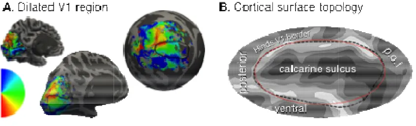
Figure 1.
Cortical surface atlas space.
(left), inflated (center), and spherical (right) hemisphere of a single subject. The black line shows the Hinds et al. [6] V1 outline throughout. (B) Cortical folding and landmarks around area V1. The cal
are indicated. The red ellipse defines the border of the algebraic template. illustrates the projection of the visual field onto this patch of cortex.
22
Cortical surface atlas space. (A) Polar angle assignment is plotted on the folded (left), inflated (center), and spherical (right) hemisphere of a single subject. The black line shows the Hinds et al. [6] V1 outline throughout. (B) Cortical folding and landmarks around area V1. The calcarine sulcus, and parieto-occipital fissure (p.o.f.) are indicated. The red ellipse defines the border of the algebraic template.
illustrates the projection of the visual field onto this patch of cortex.
(A) Polar angle assignment is plotted on the folded (left), inflated (center), and spherical (right) hemisphere of a single subject. The black line shows the Hinds et al. [6] V1 outline throughout. (B) Cortical folding and
Figure 2.
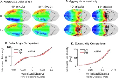
Polar angle prediction. (A) Aggregate polar angle data of 18 of the 19 subjects shown visual stimuli within 10º of fixation (one significant outlier excluded). White asterisk is the foveal confluence; black dotted line is the Hinds et al. V1 border [6]. (B
Algebraic template, fit to the aggregate polar angle map. (C) Absolute residual error between the template fit and aggregate data. (D) Median absolute prediction error across vertices and subjects by template polar angle. The median error (grey), is fit by a fifth-order polynomial (black) with the similarly fit upper and lower quartiles defining the border of the pink region. (E) Contour histogram of all vertices from 10° dataset subjects, binned by measured polar angle and superior
the template space. The template fit is shown in red. Each contour line corresponds to ~2,000 vertices. (F) Corresponding contour histogram from 20° dataset subjects. The template fit to the 20° dataset is in pink, and the fit to the 10°
reproduced from Fig 2E in red. Each contour line corresponds to ~700 vertices. Inset is the aggregate map for the 20° dataset.
aggregates and fits by hemisphere
23
(A) Aggregate polar angle data of 18 of the 19 subjects shown visual stimuli within 10º of fixation (one significant outlier excluded). White asterisk is the foveal confluence; black dotted line is the Hinds et al. V1 border [6]. (B
Algebraic template, fit to the aggregate polar angle map. (C) Absolute residual error between the template fit and aggregate data. (D) Median absolute prediction error across vertices and subjects by template polar angle. The median error (grey), is fit
order polynomial (black) with the similarly fit upper and lower quartiles defining the border of the pink region. (E) Contour histogram of all vertices from 10° dataset subjects, binned by measured polar angle and superior-inferior position in
he template space. The template fit is shown in red. Each contour line corresponds to ~2,000 vertices. (F) Corresponding contour histogram from 20° dataset subjects. The template fit to the 20° dataset is in pink, and the fit to the 10° dataset is
ed from Fig 2E in red. Each contour line corresponds to ~700 vertices. Inset is the aggregate map for the 20° dataset. Figure S2A presents the polar angle
gregates and fits by hemisphere.
(A) Aggregate polar angle data of 18 of the 19 subjects shown visual stimuli within 10º of fixation (one significant outlier excluded). White asterisk is the foveal confluence; black dotted line is the Hinds et al. V1 border [6]. (B) Algebraic template, fit to the aggregate polar angle map. (C) Absolute residual error between the template fit and aggregate data. (D) Median absolute prediction error across vertices and subjects by template polar angle. The median error (grey), is fit
order polynomial (black) with the similarly fit upper and lower quartiles defining the border of the pink region. (E) Contour histogram of all vertices from 10°
inferior position in he template space. The template fit is shown in red. Each contour line corresponds to ~2,000 vertices. (F) Corresponding contour histogram from 20° dataset subjects.
dataset is
Figure 3.
Eccentricity prediction. (A) Aggregate eccentricity
visual stimuli within 10º of fixation. White asterisk is the foveal confluence; black dotted line is the Hinds et al. V1 border [6]. (B) Algebraic model, fit to the aggregate eccentricity map, after excluding those points wi
Absolute residual error between the template fit and aggregate data. (D) Median absolute prediction error across vertices and subjects by template eccentricity. The median error (grey), is fit by a fifth
upper and lower quartiles defining the border of the pink region. (E) Contour
histogram of all vertices from 10° dataset subjects, binned by measured eccentricity and posterior-anterior position in the template space. The exponenti
shown in red. Each contour line corresponds to ~2,000 vertices. (F) Corresponding contour histogram from 20° dataset subjects. The template fit to the 20° dataset is in pink, and the fit to the 10°
line corresponds to ~800 vertices. Inset is the aggregate map for the 20° dataset. Figure S2B presents the polar angle aggregates and fits by hemisphere
24
(A) Aggregate eccentricity data of subjects (n = 19) shown visual stimuli within 10º of fixation. White asterisk is the foveal confluence; black dotted line is the Hinds et al. V1 border [6]. (B) Algebraic model, fit to the aggregate eccentricity map, after excluding those points with values ≤2.5° and ≥8°. (C)
Absolute residual error between the template fit and aggregate data. (D) Median absolute prediction error across vertices and subjects by template eccentricity. The median error (grey), is fit by a fifth-order polynomial (black) with the similarly fit upper and lower quartiles defining the border of the pink region. (E) Contour
histogram of all vertices from 10° dataset subjects, binned by measured eccentricity anterior position in the template space. The exponential template fit is shown in red. Each contour line corresponds to ~2,000 vertices. (F) Corresponding contour histogram from 20° dataset subjects. The template fit to the 20° dataset is in pink, and the fit to the 10° dataset is reproduced from Fig 2E in red. Each contour line corresponds to ~800 vertices. Inset is the aggregate map for the 20° dataset.
S2B presents the polar angle aggregates and fits by hemisphere
data of subjects (n = 19) shown visual stimuli within 10º of fixation. White asterisk is the foveal confluence; black dotted line is the Hinds et al. V1 border [6]. (B) Algebraic model, fit to the aggregate
≤2.5° and ≥8°. (C) Absolute residual error between the template fit and aggregate data. (D) Median absolute prediction error across vertices and subjects by template eccentricity. The
) with the similarly fit upper and lower quartiles defining the border of the pink region. (E) Contour
histogram of all vertices from 10° dataset subjects, binned by measured eccentricity al template fit is shown in red. Each contour line corresponds to ~2,000 vertices. (F) Corresponding contour histogram from 20° dataset subjects. The template fit to the 20° dataset is
d. Each contour line corresponds to ~800 vertices. Inset is the aggregate map for the 20° dataset.
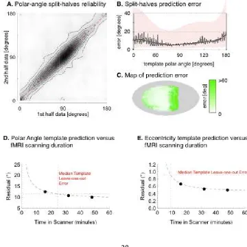
Figure 4.
Split-halves reliability of eccentricity.
eccentricity measured for each vertex for each subject from the first half of each ~30 minute scan against the eccentricity derived from the same vertex during the second half-scan. Each contour line corresponds to ~
split-halves error across vertices and subjects by template eccentricity. The median error (grey), is fit by a fifth
lower quartiles defining the border of the pin residuals between first-
cortical surface. Figure S3 presents the corresponding measurements for polar angle.
25
halves reliability of eccentricity.(A) A split-halves analysis plotted the
eccentricity measured for each vertex for each subject from the first half of each ~30 minute scan against the eccentricity derived from the same vertex during the second
scan. Each contour line corresponds to ~4,100 vertices (B) Median absolute halves error across vertices and subjects by template eccentricity. The median error (grey), is fit by a fifth-order polynomial (black) with the similarly fit upper and lower quartiles defining the border of the pink region. (C) Test-retest absolute
and second-half measurements for each vertex shown on the S3 presents the corresponding measurements for polar angle.
halves analysis plotted the
eccentricity measured for each vertex for each subject from the first half of each ~30 minute scan against the eccentricity derived from the same vertex during the second
4,100 vertices (B) Median absolute halves error across vertices and subjects by template eccentricity. The median
order polynomial (black) with the similarly fit upper and retest absolute
Figure S1.
Figure 1 presents the projection of ret
surface containing striate cortex. Shown here is a projection of the visual field (A) onto the cortical surface (B).
the apparent magnification about t
expansion of the cortical surface along the depths of the calcarine sulcus during cortical inflation and projection to a two
26
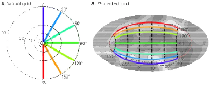
Figure 1 presents the projection of retinotopic mapping data onto a patch of cortical surface containing striate cortex. Shown here is a projection of the visual field (A) onto the cortical surface (B). Projected grid on the cortical surface. Note that some of the apparent magnification about the horizontal meridian is a consequence of
expansion of the cortical surface along the depths of the calcarine sulcus during cortical inflation and projection to a two-dimensional surface.
inotopic mapping data onto a patch of cortical surface containing striate cortex. Shown here is a projection of the visual field (A)
. Note that some of he horizontal meridian is a consequence of
Figure S2.
(A) Polar angle and (B) eccentricity aggregate
of all subjects shown stimuli out to 10° and 20° of eccentricity. (C) The average across subject polar angle and (D) eccentricity template fits, plotted as a prediction of polar angle or eccentricity against a normal
Data is plotted in black/gray for the left hemisphere, and red/pink for the right hemisphere.The thick lines indicate the template predictions in terms of normalized distance from the calcarine sulcus (polar angle) a
while the shaded regions indicate standard errors across the population of 25 subjects.
27
(A) Polar angle and (B) eccentricity aggregate data for the left and right hemispheres of all subjects shown stimuli out to 10° and 20° of eccentricity. (C) The average across subject polar angle and (D) eccentricity template fits, plotted as a prediction of polar angle or eccentricity against a normalized iso-eccentric or iso
Data is plotted in black/gray for the left hemisphere, and red/pink for the right hemisphere.The thick lines indicate the template predictions in terms of normalized distance from the calcarine sulcus (polar angle) and the occipital pole (eccentricity) while the shaded regions indicate standard errors across the population of 25
data for the left and right hemispheres of all subjects shown stimuli out to 10° and 20° of eccentricity. (C) The average across subject polar angle and (D) eccentricity template fits, plotted as a prediction
eccentric or iso-angular axis. Data is plotted in black/gray for the left hemisphere, and red/pink for the right hemisphere.The thick lines indicate the template predictions in terms of normalized
Figure S3.
(A) Contour histogram of all vertices for the 10° dataset determined by calculation of polar angle separately for each half of the fMRI scan. Each contour line corresponds to ~4,100 vertices (B) Median absolute split
subjects by template eccentricity. The median error (grey), is fit by a fifth polynomial (black) with
of the pink region. (C) Test
measurements for each vertex shown on the cortical surface. The lower two panels present the median absolute err
(D) polar angle and (E) eccentricity derived from an fMRI, retinotopic mapping session of a given duration (x
minute scan from the same individual. A decaying polynomial of t
was fit to the data and is plotted with a dashed black line. The performance of our template across the population of 19 other subjects shown stimulus out to 10° of eccentricity is indicated by a dotted red cross
the median absolute leave
subject) to the left-out subject. The corresponding x
scanner time required in the example subject to obtain a precision of retino mapping equivalent to the anatomical, template approach.
28
(A) Contour histogram of all vertices for the 10° dataset determined by calculation of y for each half of the fMRI scan. Each contour line corresponds to ~4,100 vertices (B) Median absolute split-halves error across vertices and
subjects by template eccentricity. The median error (grey), is fit by a fifth
polynomial (black) with the similarly fit upper and lower quartiles defining the border of the pink region. (C) Test-retest absolute residuals between first- and second measurements for each vertex shown on the cortical surface.
The lower two panels present the median absolute error (y-axis) in measurement of (D) polar angle and (E) eccentricity derived from an fMRI, retinotopic mapping session of a given duration (x-axis) as determined by comparison to a separate, 48 minute scan from the same individual. A decaying polynomial of the form c1 + c2 x was fit to the data and is plotted with a dashed black line. The performance of our template across the population of 19 other subjects shown stimulus out to 10° of eccentricity is indicated by a dotted red cross-hairs, the y-value of which indicates the median absolute leave-one-out error from the template (made with all but one
out subject. The corresponding x-value indicates the amount of scanner time required in the example subject to obtain a precision of retino
mapping equivalent to the anatomical, template approach.
(A) Contour histogram of all vertices for the 10° dataset determined by calculation of y for each half of the fMRI scan. Each contour line corresponds
halves error across vertices and subjects by template eccentricity. The median error (grey), is fit by a fifth-order
milarly fit upper and lower quartiles defining the border and second-half
axis) in measurement of (D) polar angle and (E) eccentricity derived from an fMRI, retinotopic mapping
axis) as determined by comparison to a separate, 48 he form c1 + c2 x-k was fit to the data and is plotted with a dashed black line. The performance of our template across the population of 19 other subjects shown stimulus out to 10° of
hich indicates out error from the template (made with all but one
29
CHAPTER 3 - The Fine-Scale Functional Correlation of Striate Cortex in
Sighted and Blind People
Butt OH & Benson NC; Datta R; Aguirre GK. (2013). Journal of Neuroscience,
33(41):16209-19.
Abstract
To what extent are spontaneous neural signals within striate cortex organized by
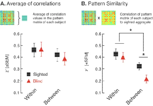
vision? We examined the fine-scale pattern of striate cortex correlations within and
between hemispheres in rest-state BOLD fMRI data from sighted and blind people. In
the sighted, we find that cortico-cortico correlation is well modeled as a Gaussian
point-spread function across millimeters of striate cortical surface, rather than
degrees of visual angle. Blindness produces a subtle change in the pattern of
fine-scale striate correlations between hemispheres. Across participants blind before the
age of 18, the degree of pattern alteration covaries with the strength of long-range
correlation between left striate cortex and Broca’s area. This suggests that early
blindness exchanges local, vision-driven pattern synchrony of the striate cortices for
long-range functional correlations potentially related to cross-modal representation.
Introduction
Spontaneous neural activity is observed in the absence of structured sensory input or
motor output (Arieli et al., 1995,1996, Fiser et al., 2004, He et al., 2008, 2010) and
these signals display informative spatiotemporal synchrony (Fox et al., 2007). Slow
fluctuations in the BOLD fMRI signal measured at rest reflect neural activity (Biswal
30
(Hagmann et al., 2008, Greicius et al., 2009, van den Heuvel et al., 2009, Honey et
al., 2009). Recent work has examined correlation structure at a fine (millimeter)
scale, for example revealing that the pattern of resting-state correlations in the
somatosensory cortex of the squirrel monkey reflects the representation of individual
digits of the hand (Chen et al., 2012). This scale of analysis allows for tests of the
relationship between the spontaneous signals and the functional organization of
sensory cortex.
In visual cortex, the fine-scale structure of correlations measured with functional
MRI reveals a pattern aligned with retinotopy (Heinzle et al., 2011, Jo et al., 2012),
which is the mapping of the visual field to the two-dimensional surface of cortex.
Spontaneous neural signals may be organized by this fundamental, functional
property of visual cortex, linking together neurons that share representation of
similar positions in the visual world. A limitation to such claims, however, is that
these studies have generally not tested if the pattern of correlations reflect visual
function per se, or are instead an intrinsic property of cortex that happens to align
with retinotopy. This is a plausible concern as retinotopic organization is a spatially
smooth gradient of eccentricity and polar angle visual field position across the
cortex, and thus could resemble other spatial gradients of spontaneous neural
activity, or even non-neural physiologic processes. The current study asks if the
fine-scale properties of functional correlation reflect subtle, specific properties of
retinotopic organization. We examine in particular the first cortical visual area, the
striate cortex. We test if resting-state correlations display “magnification” along the
eccentricity axis and enhanced correlation along the vertical meridian between
hemispheres, both specific functional properties of the visual cortex.
We then examine how the pattern of fine-scale correlation is altered in blindness.
31
and function (Bendy et al., 2011; Cohen et al., 1999; Liu et al., 2007; Sadato et al.,
2002; Watkins et al., 2012) of striate cortex is altered in blind people.
To date, studies of resting-state signals in blind people have only examined
whole-region correlations, finding a reduction in correlation of extra-striate (although
not striate) occipital cortex between hemispheres (Watkins et al., 2012). In animal
studies, visual experience drives the pruning of diffuse synaptic connections in the
occipital cortex (Innocenti & Price, 2005), leading to the prediction of an altered
(perhaps broadened) pattern of fine-scale correlation in the visual cortex of blind
humans.
To allow comparisons between blind and sighted subjects within a common
framework, we make use of recent methodological advances that establish
hemispheric homology and functional assignment based upon cortical surface
topology. Gray matter surface alignment using gyral landmarks (Fischl et al., 1999)
allows for accurate prediction not only of the boundaries of striate cortex (Hinds et
al., 2008) but the assignment of retinotopic polar angle and eccentricity (Benson et
al., 2012).
Material and Methods
Subjects
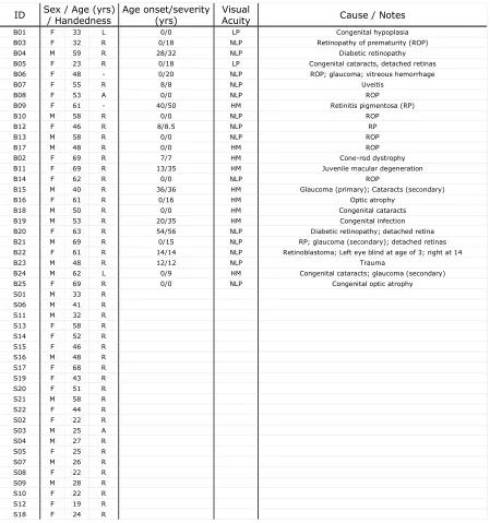
A total of 47 subjects participated in resting-state experiments (Table 1; 21 females
and 26 males), 25 of whom had severe or complete vision loss, and 22 normally
sighted controls. The blind participants (mean age of 54) varied in the age at which
they lost vision (Table 1), with 16 losing sight before the age of 18. The 22 sighted
subjects had normal or corrected-to-normal visual acuity and were on average
younger (mean age of 37). As normal aging is associated with changes in resting