University of Pennsylvania
ScholarlyCommons
Publicly Accessible Penn Dissertations
1-1-2015
Bayesian Network Games
Ceyhun Eksin
University of Pennsylvania, [email protected]
Follow this and additional works at:http://repository.upenn.edu/edissertations
Part of theElectrical and Electronics Commons
This paper is posted at ScholarlyCommons.http://repository.upenn.edu/edissertations/1052
For more information, please [email protected]. Recommended Citation
Eksin, Ceyhun, "Bayesian Network Games" (2015).Publicly Accessible Penn Dissertations. 1052.
Bayesian Network Games
Abstract
This thesis builds from the realization that Bayesian Nash equilibria are the natural definition of optimal behavior in a network of distributed autonomous agents. Game equilibria are often behavior models of competing rational agents that take actions that are strategic reactions to the predicted actions of other players. In autonomous systems however, equilibria are used as models of optimal behavior for a different reason: Agents are forced to play strategically against inherent uncertainty. While it may be that agents have
conflicting intentions, more often than not, their goals are aligned. However, barring unreasonable accuracy of environmental information and unjustifiable levels of coordination, they still can't be sure of what the actions of other agents will be. Agents have to focus their strategic reasoning on what they believe the information available to other agents is, how they think other agents will respond to this hypothetical information, and choose what they deem to be their best response to these uncertain estimates. If agents model the behavior of each other as equally strategic, the optimal response of the network as a whole is a Bayesian Nash equilibrium. We say that the agents are playing a Bayesian network game when they repeatedly act according to a stage Bayesian Nash equilibrium and receive information from their neighbors in the network.
The first part of the thesis is concerned with the development and analysis of algorithms that agents can use to compute their equilibrium actions in a game of incomplete information with repeated interactions over a network. In this regard, the burden of computing a Bayesian Nash equilibrium in repeated games is, in general, overwhelming. This thesis shows that actions are computable in the particular case when the local information that agents receive follows a Gaussian distribution and the game's payoff is represented by a utility function that is quadratic in the actions of all agents and an unknown parameter. This solution comes in the form of the Quadratic Network Game filter that agents can run locally, i.e., without access to all private signals, to
compute their equilibrium actions. For the more generic payoff case of Bayesian potential games, i.e., payoffs represented by a potential function that depends on population actions and an unknown state of the world, distributed versions of fictitious play that converge to Nash equilibrium with identical beliefs on the state are derived. This algorithm highlights the fact that in order to determine optimal actions there are two problems that have to be solved: (i) Construction of a belief on the state of the world and the actions of other agents. (ii) Determination of optimal responses to the acquired beliefs. In the case of symmetric and strictly
supermodular games, i.e., games with coordination incentives, the thesis also derives qualitative properties of Bayesian network games played in the time limit. In particular, we ask whether agents that play and observe equilibrium actions are able to coordinate on an action and learn about others' behavior from only observing peers' actions. The analysis described here shows that agents eventually coordinate on a consensus action.
The second part of this thesis considers the application of the algorithms developed in the first part to the analysis of energy markets. Consumer demand profiles and fluctuating renewable power generation are two main sources of uncertainty in matching demand and supply in an energy market. We propose a model of the electricity market that captures the uncertainties on both, the operator and the user side. The system operator (SO) implements a temporal linear pricing strategy that depends on real-time demand and renewable generation in the considered period combining Real-Time Pricing with Time-of-Use Pricing. The announced pricing strategy sets up a noncooperative game of incomplete information among the users with
policies yield close to optimal welfare values while improving these practical objectives. We then analyze the sensitivity of the proposed pricing schemes to user behavior and information exchange models. Selfish, altruistic and welfare maximizing user behavior models are considered. Furthermore, information exchange models in which users only have private information, communicate or receive broadcasted information are considered. For each pair of behavior and information exchange models, rational price anticipating
consumption strategy is characterized. In all of the information exchange models, equilibrium actions can be computed using the Quadratic Network Game filter. Further experiments reveal that communication model is beneficial for the expected aggregate payoff while it does not affect the expected net revenue of the system operator. Moreover, additional information to the users reduces the variance of total consumption among runs, increasing the accuracy of demand predictions.
Degree Type
Dissertation
Degree Name
Doctor of Philosophy (PhD)
Graduate Group
Electrical & Systems Engineering
First Advisor
Alejandro Ribeiro
Second Advisor
Rakesh Vohra
Keywords
Distributed autonomous systems, Game theory, Multi-agent systems, Smart grids
Subject Categories
BAYESIAN NETWORK GAMES
Ceyhun Eksin
A DISSERTATION
in
Electrical & Systems Engineering
Presented to the Faculties of the University of Pennsylvania in Partial
Fulfillment of the Requirements for the Degree of Doctor of Philosophy
2015
Alejandro Ribeiro, Professor Electrical & Systems Engineering
Supervisor of Dissertation
Saswati Sarkar, Professor Electrical & Systems Engineering
Graduate Group Chairperson
Dissertation committee:
Rakesh Vohra, Chair of the Committee, Professor, Electrical & Systems
Engineering
Alejandro Ribeiro, Professor, Electrical & Systems Engineering
Ali Jadbabaie, Professor, Electrical & Systems Engineering
Jeff S. Shamma, Professor, Electrical & Computer Engineering, Georgia Institute
BAYESIAN NETWORK GAMES
COPYRIGHT
2015
Acknowledgments
Like in any rite of passage, what makes my graduate studies at the University of
Pennsylvania memorable and transforming is neither the beginning nor the end but
it is the experience itself. This is a tribute to the people that influenced my Ph.D.
life.
First and foremost, I would like to express my deepest gratitude to my advisor
Professor Alejandro Ribeiro for his patience, passion, guidance and support. Besides
many of his teachings and ideas that I will benefit from in the years to come, his
guidance style will be a source of inspiration. Finally, I thank him for accepting me
as his student after my third year as a graduate student.
Special thanks go to professors Rakesh Vohra, Ali Jadbabaie, and Jeff S. Shamma,
for graciously agreeing to serve on my committee. I am grateful to constructive
suggestions and helpful comments of Prof. Rakesh Vohra on my thesis that have
pushed me to think deeper about my work. I also would like to acknowledge Prof.
Ali Jadbabaie for being a supportive collaborator. I extend my appreciation to Prof.
Jeff S. Shamma for his encouragement and support. I am doubly thankful to Jeff for
traveling to attend my Ph.D. proposal.
Academic life is social. During the course of my Ph.D. life, I benefited greatly
from the academic friendship of Dr. Pooya Molavi and Prof. Hakan Deli¸c. For this,
I would like to thank Pooya for our many discussions on Bayesian Network Games,
and for being a true collaborator and friend. I am deeply indebted to Hakan for
grids. Without his presence in my academic life, Chapters 5 and 6 of this thesis
would not have existed. I also would like to thank my collaborators at NEC Labs
America, Ali Hooshmand and Ratnesh Sharma.
I will remember my days as a graduate student with all the people that
accom-panied me. I thank all the people, who dwelled in the ACASA lab and in the room
Moore 306, for their friendship and support in my years of graduate school. Thank
you for your company, it has been a pleasure. I also would like to thank Atahan
A˘gralı, Sean Arlauckas, Sina Teoman Ate¸s, Taygun Ba¸saran, Doruk Baykal, Ba¸sak
Can, Chinwendu Enyioha, Burcu Kement, Chris P. Morgan, Ekim Cem Muyan,
Daniel Neuhann, Miroslav Pajic, Necati Tereya˘go˘glu, and many other friends who
have made Philadelphia a home. I extend my special thanks to my friends in Istanbul
who have always welcomed me back during my travels back.
Last but not the least, I thank my family: my parents, Aydan and Ibrahim, my
brother Orhun, my grandparents, and Defne for their love and support. You shaped
my heart, and my mind. Defne, aramızdaki ¸su g¨on¨ulden g¨on¨ule giden g¨or¨ulmeyen
ABSTRACT
BAYESIAN NETWORK GAMES
Ceyhun Eksin
Alejandro Ribeiro
This thesis builds from the realization that Bayesian Nash equilibria are the
nat-ural definition of optimal behavior in a network of distributed autonomous agents.
Game equilibria are often behavior models of competing rational agents that take
actions that are strategic reactions to the predicted actions of other players. In
au-tonomous systems however, equilibria are used as models of optimal behavior for a
different reason: Agents are forced to play strategically against inherent uncertainty.
While it may be that agents have conflicting intentions, more often than not, their
goals are aligned. However, barring unreasonable accuracy of environmental
infor-mation and unjustifiable levels of coordination, they still can’t be sure of what the
actions of other agents will be. Agents have to focus their strategic reasoning on
what they believe the information available to other agents is, how they think other
agents will respond to this hypothetical information, and choose what they deem to
be their best response to these uncertain estimates. If agents model the behavior of
each other as equally strategic, the optimal response of the network as a whole is a
Bayesian Nash equilibrium. We say that the agents are playing a Bayesian network
game when they repeatedly act according to a stage Bayesian Nash equilibrium and
receive information from their neighbors in the network.
The first part of the thesis is concerned with the development and analysis of
algorithms that agents can use to compute their equilibrium actions in a game of
in-complete information with repeated interactions over a network. In this regard, the
burden of computing a Bayesian Nash equilibrium in repeated games is, in general,
when the local information that agents receive follows a Gaussian distribution and
the game’s payoff is represented by a utility function that is quadratic in the actions
of all agents and an unknown parameter. This solution comes in the form of the
Quadratic Network Game filter that agents can run locally, i.e., without access to
all private signals, to compute their equilibrium actions. For the more generic payoff
case of Bayesian potential games, i.e., payoffs represented by a potential function
that depends on population actions and an unknown state of the world, distributed
versions of fictitious play that converge to Nash equilibrium with identical beliefs on
the state are derived. This algorithm highlights the fact that in order to determine
optimal actions there are two problems that have to be solved: (i) Construction of a
belief on the state of the world and the actions of other agents. (ii) Determination
of optimal responses to the acquired beliefs. In the case of symmetric and strictly
supermodular games, i.e., games with coordination incentives, the thesis also derives
qualitative properties of Bayesian network games played in the time limit. In
par-ticular, we ask whether agents that play and observe equilibrium actions are able to
coordinate on an action and learn about others’ behavior from only observing peers’
actions. The analysis described here shows that agents eventually coordinate on a
consensus action.
The second part of this thesis considers the application of the algorithms
devel-oped in the first part to the analysis of energy markets. Consumer demand profiles
and fluctuating renewable power generation are two main sources of uncertainty in
matching demand and supply in an energy market. We propose a model of the
elec-tricity market that captures the uncertainties on both, the operator and the user
side. The system operator (SO) implements a temporal linear pricing strategy that
depends on real-time demand and renewable generation in the considered period
sets up a noncooperative game of incomplete information among the users with
het-erogeneous but correlated consumption preferences. An explicit characterization of
the optimal user behavior using the Bayesian Nash equilibrium solution concept is
derived. This explicit characterization allows the SO to derive pricing policies that
influence demand to serve practical objectives such as minimizing peak-to-average
ratio or attaining a desired rate of return. Numerical experiments show that the
pricing policies yield close to optimal welfare values while improving these practical
objectives. We then analyze the sensitivity of the proposed pricing schemes to user
behavior and information exchange models. Selfish, altruistic and welfare
maximiz-ing user behavior models are considered. Furthermore, information exchange models
in which users only have private information, communicate or receive broadcasted
information are considered. For each pair of behavior and information exchange
models, rational price anticipating consumption strategy is characterized. In all of
the information exchange models, equilibrium actions can be computed using the
Quadratic Network Game filter. Further experiments reveal that communication
model is beneficial for the expected aggregate payoff while it does not affect the
ex-pected net revenue of the system operator. Moreover, additional information to the
users reduces the variance of total consumption among runs, increasing the accuracy
Contents
Acknowledgments iv
1 The Interactive Decision-Making Problem 1
1.1 Decision-Making Environment . . . 4
1.2 Bayesian Network Game . . . 8
1.2.1 A BNG example . . . 13
1.2.2 Discussions on the BNG . . . 17
1.3 Roadmap and Contributions . . . 20
1.3.1 Rational behavior models . . . 20
1.3.2 Bounded rational behavior models . . . 24
1.3.3 Demand response in smart grids . . . 27
1.4 Interactive decision-making models in the literature . . . 28
I
Interactive Decision-Making Models in Bayesian
Net-work Games
33
2 Bayesian Quadratic Network Games 34 2.1 Introduction . . . 342.2 Gaussian Quadratic Games . . . 36
2.2.1 Bayesian Nash equilibria . . . 38
2.3 Propagation of probability distributions . . . 41
2.4 Quadratic Network Game Filter . . . 52
2.5 Vector states and vector observations . . . 58
2.6 Cournot Competition . . . 65
2.6.1 Learning in Cournot competition . . . 67
2.7 Coordination Game . . . 70
2.7.1 Learning in coordination games . . . 71
2.8 Summary . . . 73
3 Distributed Fictitious Play 75 3.1 Introduction . . . 75
3.2.1 Fictitious play . . . 82
3.2.2 Distributed fictitious play . . . 83
3.2.3 State Relevant Information . . . 85
3.3 Convergence in Symmetric Potential Games with Incomplete Infor-mation . . . 86
3.4 Distributed Fictitious Play: Histogram Sharing . . . 92
3.5 Simulations . . . 96
3.5.1 Beauty contest game . . . 97
3.5.2 Target covering game . . . 100
3.6 Summary . . . 103
4 Learning to Coordinate in Social Networks 106 4.1 Introduction . . . 106
4.2 Model . . . 110
4.2.1 The game . . . 110
4.2.2 Equilibrium . . . 112
4.2.3 Remarks on the model . . . 113
4.3 Main Result . . . 114
4.4 Discussion . . . 118
4.4.1 Consensus . . . 118
4.4.2 Extensions . . . 121
4.5 Symmetric Supermodular Games . . . 122
4.5.1 Currency attacks . . . 122
4.5.2 Bertrand competition . . . 123
4.5.3 Power control in wireless networks . . . 124
4.5.4 Arms race . . . 125
4.6 Summary . . . 125
II
Demand Response Management in Smart Grids
127
5 Demand Response Management in Smart Grids with Heteroge-neous Consumer Preferences 128 5.1 Introduction . . . 1295.2 Smart Grid Model . . . 131
5.2.1 System operator model . . . 132
5.2.2 Power consumer . . . 135
5.3 Customers’ Bayesian Game . . . 137
5.4 Numerical Examples . . . 143
5.4.1 Effect of consumption preference distribution . . . 144
5.4.2 Effect of policy parameter . . . 146
5.4.3 Effect of uncertainty in renewable power . . . 147
5.5.1 Efficient Competitive Equilibrium . . . 152
5.5.2 Analytical comparison among pricing policies . . . 156
5.5.3 Numerical comparison among pricing policies . . . 158
5.6 Discussions and Policy Implications . . . 160
6 Demand Response Management in Smart Grids with Cooperating Rational Consumers 163 6.1 Introduction . . . 163
6.2 Demand Response Model . . . 165
6.2.1 Real Time Pricing . . . 165
6.2.2 Power consumer . . . 166
6.2.3 Consumer behavior models . . . 166
6.2.4 Information exchange models . . . 167
6.3 Bayesian Nash equilibria . . . 169
6.4 Consumers’ Bayesian Game . . . 171
6.4.1 Private and Full information games . . . 178
6.5 Price taking Consumers . . . 178
6.6 Numerical Analyses . . . 180
6.6.1 Effect of consumer behavior . . . 182
6.6.2 Effect of information exchange models . . . 183
6.6.3 Effect of population size (N) . . . 184
6.6.4 Effect of renewable uncertainty . . . 187
6.7 Summary . . . 188
7 Conclusions 189 7.1 Dissertation Summary . . . 189
List of Figures
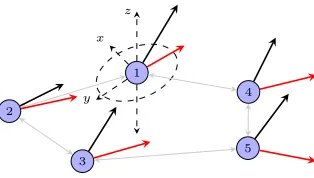
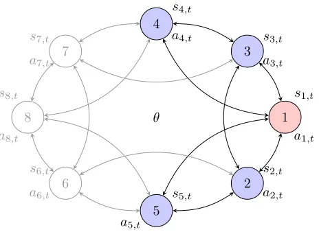
1.1 Bayesian network games. Agents want to select actions that are
op-timal with respect to an unknown state of the world and the actions taken by other agents. Although willing to cooperate, nodes are forced to play strategically because they are uncertain about what the ac-tions of other nodes are. . . 5
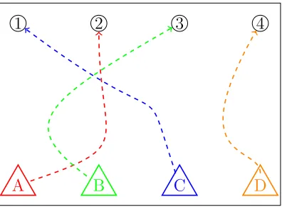
1.2 Target covering problem. 4 robots partake in covering 4 entrances of
a building. Each robot makes noisy private measurements si,t about
the locations of the entrances θ. . . 6
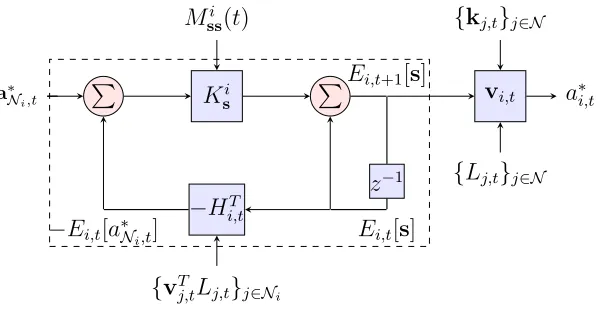
1.3 Quadratic Network Game (QNG) filter. Agents run the QNG filter to
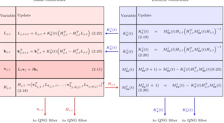
compute BNE actions in games with quadrate payoffs and Gaussian private signals. . . 21
2.1 Quadratic Network Game (QNG) filter at agenti. There are two types
of blocks, circle and rectangle. Arrows coming into the circle block are summed. The arrow that goes into a rectangle block is multiplied by the coefficient written inside the block. Inside the dashed box agent i’s mean estimate updates ons and θ are illustrated (cf. (2.42) and (2.43)). The gain coefficients for the mean updates are fed from
LMMSE block in Fig. 2. The observation matrixHi,t is fed from the
game block in Fig. 2. Agent i multiplies his mean estimate on s at
time t with action coefficient vi,t, which is fed from game block in
Fig. 2, to obtainai,t. The mean estimates Ei,t[s] andai,t can only be
calculated by agenti. . . 53
2.2 Propagation of gains required to implement the Quadratic Network
Game (QNG) filter of Fig. 2.1. Gains are separated into interacting LMMSE and game blocks. All agents perform a full network simu-lation in which they compute the gains of all other agents. This is
necessary because when we compute the play coefficients vj,t in the
game block, agentibuilds the matrix Lt that is formed by the blocks
Lj,t of all agents [cf. (2.10)]. This full network simulation is possible
2.4 Agents’ actions over time for the Cournot competition game and net-works shown in Fig. 2.3. Each line indicates the quantity produced for an individual at each stage. Actions converge to the Nash equilib-rium action of the complete information game in the number of steps equal to the diameter of the network. . . 68
2.5 Normed error in estimates of privates signals, ks−Ei,t[s]k22, for the Cournot competition game and networks shown in Fig. 2.3. Each line corresponds to an agent’s normed error in mean estimates of private signals over the time horizon. While all of the agents learn the true values of all the private signals in line and ring networks, in the star
network only the central agent learns all of the private signals. . . . 68
2.6 Mobile agents in a 3-dimensional coordination game. Agents observe
initial noisy private signals on heading and take-off angles. Red and black lines are illustrative heading and take-off angle signals,
respec-tively. Agents revise their estimates on true heading and take-off
angles and coordinate their movement angles with each other through local observations. . . 69
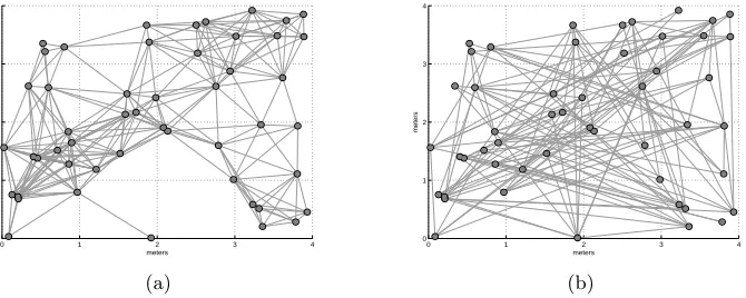
2.7 Geometric (a) and random (b) networks withN = 50 agents. Agents
are randomly placed on a 4 meter ×4 meter square. There exists an
edge between any pair of agents with distance less than 1 meter apart in the geometric network. In the random network, the connection probability between any pair of agents is independent and equal to 0.1. 72
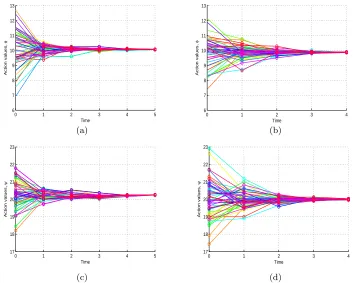
2.8 Agents’ actions over time for the coordination game and networks
shown in Fig. 2.7. Values of agents’ actions over time for heading
angle φi (top) and take-off angle ψi in geometric (left) and random
(right) networks respectively. Action consensus happens in the order
of the diameter of the corresponding networks. . . 73
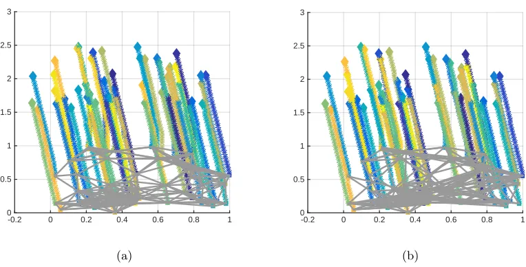
3.1 Position of robots over time for the geometric (a) and small world
3.2 Actions of robots over time for the geometric (a) and small world networks (b). Solid lines correspond to each robots’ actions over time.
The dotted dashed line is equal to value of the state of the world θ
and the dashed line is the optimal estimate of the state given all of
the signals. Agents reach consensus in the movement direction 95◦
faster in the small-world network than the geometric network. . . 98
3.3 Locations (a) and actions (b) of robots over time for the star network. There areN = 5 robots and targets. In (a), the initial positions of the robots are marked with squares. The robots’ final positions at the end of 100 steps are marked with a diamond. The crosses indicate the po-sition of the targets. Robots follow the histogram sharing distributed fictitious play presented in Section 3.4. The stars in (a) represent the position of the robots at each step of the algorithm. The solid lines in (b) correspond to the actions of robots over time. Each target is covered by a single robot before 100 steps. . . 99
3.4 Comparison of the distributed fictitious play algorithm with the
cen-tralized optimal solution. Best and worst correspond to the runs with the highest and lowest global utility in the distributed fictitious play algorithm. Out of the 50 runs, in 40 runs the algorithm converges to the highest global utility. . . 104
5.1 Illustration of information flow between the power provider and the
consumers. The SO determines the pricing policy (6.2) and broadcasts it to the users along with its prediction of renewable energy termPωh.
Selfish (6.3) users respond optimally to realize demandL∗h =P
i∈Nl ∗
ih.
The realized demand per user ¯L∗h together with realized renewable
generation term ωh determines the price at time h. . . 134
5.2 Effect of preference distribution on performance metrics: Aggregate
UtilityUh (a), total consumption Lh (b), price ph(Lh;βh, ωh) (c), and
realized rate of return rh (d). Each line represents the value of the
performance metric with respect to three values of σij ∈ {0,2,4}
as color coded in the legend of (d). Solid lines represent the average value over 100 instantiations. Dashed lines indicate the maximum and minimum values of 100 instantiations. Changes in user preferences do not affect mean rate of return of the SO. . . 143
5.3 Effect of policy parameter on performance metrics: total consumption
Lh (a), and realized rate of return rh (b). Each solid line represents
the average value (over 100 realizations) of the performance metric with respect to three values of γ ∈ {0.5,0.6,0.7} where γh = γ for
h ∈ H color coded in each figure. Dashed lines mark minimum and
5.4 Effect of prediction error of renewable power uncertainty ωh on
per-formance metrics: aggregate utilityP
h∈HUh (a) and net revenueN R
(b). In both figures, the horizontal axis shows the prediction error for the renewable term in price, that is,ωh =ωand ¯ωh = ¯ωforh∈ Hand
it showsω−ω¯. Each point in the plots corresponds to the value of the metric at a single initialization. When the realized renewable term ω
is larger than predicted ¯ω, net revenue increases. Given a fixed error in renewable prediction, aggregate utility is larger and net revenue is smaller when predicted value ¯ω is smaller. . . 146
5.5 Comparison of different pricing schemes with respect to Welfare W
(a), PAR of Total Consumption (b), Total ConsumptionP
h∈HLh (c).
In (a)-(c), each point corresponds to the value of the metric for that scenario and dashed lines correspond to the average value of these points over all scenarios with colors associating the point with the pricing scheme in the legend. The PAR-minimizing policy performs better than others in minimizing PAR of consumption while at the same time being comparable to the competitive equilibrium pricing model (CCE) in welfare. . . 156
6.1 Total consumption over time for Γ =S and Ω ∈{P, AS, B} for N =
{3,5,10,15} population size. For the AS information each plot
cor-responds to a geometric communication network of N consumers on
a 3 mile×5 mile area with a threshold connectivity of 2 miles. When the network is connected, AS information exchange model converges to the B information exchange model in the number of steps equal to the diameter of the network. . . 185
6.2 Expected welfare loss EW L/N per capita for population size N ∈
{10,100,500,1000} with respect to preference correlation coefficient
σij ∈ {0,0.8,1.6,2.4,3.2,4}. Expected welfare loss EW Lis the
differ-ence in expected welfare when Γ =W, Ω =B and when Γ =S, Ω =P. Expectation of welfare is computed by averaging 20 runs with
instan-tiations of the preference profile g and the renewable sources ω. As
the population size increases theEW L/N disappears. . . 186
6.3 Effect of mean estimate of renewable energy ¯ω on total consumption
per capita EL/N¯ (a) and welfare EW (b). The renewable term ¯ω
takes values in{−2,−1,0,1,2}and the correlation coefficient is fixed
at σij = 2.4. For each anticipatory behavior model Γ ∈{S,U,W}
Chapter 1
The Interactive Decision-Making
Problem
In a social system, actions of individuals create cascading effects on the entire society
as each action not only affect the fundamentals that it is acting upon but also change
the perceptions of the members of the society. For instance, in the stock market,
agents with uncertainty on the true value of the share take actions that affect the
profits of all the agents while, at the same time, these actions carry information
about actors’ beliefs on the true value of the share affecting observers’ beliefs on the
value of the share. The change in the belief of the observers ends the first cycle of
the cascading effect and possibly causes the observers to act differently in the future
starting the second cycle of the cascading effect. When we consider social systems,
our goal is descriptive, that is, we model to understand, whereas, in technological
settings, we build models to design. Regardless of the goal, in a technological
so-ciety, e.g., a distributed autonomous system where a team of robots want to act in
coordination, our modeling should incorporate the cascading effect as information
the unknown state of the world. Common to both social and technological societies
is that both information and decision-making is decentralized. The sequential
in-dividual decision-making modeling problem that we encounter in these settings we
dub the interactive decision-making problem.
This dissertation’s focus is the interactive decision-decision making problem in
which agents with identical or differing payoffs that depend on the actions of others
and an uncertain state of the world sequentially make decisions. While we do not
enforce that agents have identical payoffs in the setup, in many technological
set-tings, there exists a global objective that all agents would like to jointly maximize.
For instance, in a wireless communication network, agents would like to maximize
throughput or allocate resources efficiently, or in a distributed autonomous system a
team of robots may want to move in alignment with each other. The maximization
of the payoffs could be relatively easy if agents had common information or there
ex-isted a centralized decision maker that dictates the behavior of each agent. However,
neither the common information nor the centralized decision-making is a reasonable
model of the environment in large scale systems with many agents. A reasonable
model of information acquisition is that agents possibly receive private information
about the state, and exchange messages with their neighbors over a network. What
information should be exchanged with the messages and how agents process their
information are the modeling problems we address in this dissertation.
Given the decentralized information, Bayesian Nash equilibrium (BNE) is the
rational behavior model that maximizes expected current individual payoff. In
BNE behavior, individuals have the correct understanding of the environment, are
Bayesian in processing information, and play optimally with respect to their Bayesian
beliefs. Game equilibria are behavioral models of competing agents that take actions
systems however, BNE is a model of optimal behavior for a different reason: Agents
are forced to play strategically against inherent uncertainty. While it may be that
agents have conflicting intentions, more often than not, their goals are aligned.
How-ever, barring unreasonable accuracy of environmental information and unjustifiable
levels of coordination, they still can’t be sure of what the actions of other agents
will be. Agents have to focus their strategic reasoning on what they believe the
information available to other agents is, how they think other agents will respond to
this hypothetical information, and choose what they deem to be their best response
to these uncertain estimates. If an agent models the behavior of other agents as
equally strategic, the optimal response of the network as a whole is a BNE. When
agents play according to a stage BNE strategy profile at each decision-making time,
we say that the agents are playing a Bayesian network game (BNG).
The research in this thesis contributes to the interactive decision-making
prob-lem in Bayesian network games in two theoretical thrusts: 1) rational behavior and
2) bounded rational behavior. In the rational behavior thrust our goal is to design
tractable local algorithms for computation of stage BNE behavior in BNG and to
analyze asymptotic outcomes of BNG. In the bounded rational behavior model our
goal is to overcome the computational demand of BNE by proposing simple
algo-rithms that approximates BNE behavior and becomes asymptotically rational. Our
application domain in these two theoretical thrusts is distributed autonomous
sys-tems. In the second part of the thesis, we focus on applying the rational behavior
model to smart grid power systems.
In the rest of this chapter, we first describe the interactive decision-making
envi-ronment and formalize the BNG, and then provide an overview of each thrust and
1.1
Decision-Making Environment
The interactive-decision making environment considered in this dissertation,
de-picted in Figure 1.1, comprises an unknown state of the world θ ∈ Θ and a group
of agents N ={1, . . . , N}whose interactions are characterized by a network G with node set N and edge setE,G = (N,E). At subsequent points in timet= 0,1,2, . . .,
agents in the network observe private signals si,t that possibly carry information
about the state of the world θ and decide on an action ai,t belonging to some
com-mon compact metric action spaceAthat they deem optimal with respect to a utility
function of the form
ui ai,t, a−i,t, θ
. (1.1)
Besides his action ai,t, the utility of agent i depends on the state of the world θ and
the actions a−i,t := {aj,t}j∈N \i of all other agents in the network. For example, in
a social setting where customers decide how much to use a service, the state of the
world θ may represent the inherent value of a service, the private signals si,t may
represent quality perceptions after use, and the action ai,t may represent decisions
on how much to use the service. The utility of a person derives from the use of the
service depending not only on the inherent quality θ but also on how much others
use the service. In a technological setting where a team of robots wants to align
its movement direction, the state of the world θ may represent the unknown target
direction of movement, the private signals si,t may represent the noisy measurement
of the target direction, and the action ai,t may represent its choice of movement
direction.
Deciding optimal actions ai,t would be easy if all agents were able to coordinate
their information and their actions. All private signalssi,tcould be combined to form
θ 1
2 3 4
5
6 7
8
s1,t
a1,t
s2,t
a2,t
s3,t
a3,t
s4,t
a4,t
s5,t
a5,t
s6,t
a6,t
s7,t
a7,t
s8,t
a8,t
Figure 1.1: Bayesian network games. Agents want to select actions that are optimal with respect to an unknown state of the world and the actions taken by other agents. Although willing to cooperate, nodes are forced to play strategically because they are uncertain about what the actions of other nodes are.
used to select ai,t. Whether there is payoff dependence on others’ actions or not,
global coordination is an implausible model of behavior in social and technological
societies for two main reasons. The first reason is that the information is inherently
decentralized and combining the global information at all nodes of the network costs
time and energy. The second reason is that even if the information can be aggregated
at a central location, the solution can be computationally demanding to obtain
by the central processor. We, therefore, consider agents that act independently of
each other and couple their behavior through observations of past information from
agents in their network neighborhood Ni :={j : (j, i) ∈ E}. The network indicates
that agents are local information sources, that is, agents observe other information
shared by neighboring agents at a given time. In observing neighboring information
agents have the opportunity to learn about the private information that neighbors
are revealing. Acquiring this information alters agents’ beliefs leading to the selection
of new actions which become known at the next play prompting further reevaluation
A B C D
1 2 3 4
Figure 1.2: Target covering problem. 4 robots partake in covering 4 entrances of a
building. Each robot makes noisy private measurements si,t about the locations of
the entrances θ.
The diagram in Figure 1.1 is a generic representation of a distributed autonomous
system. The team is assigned a certain goal that depends on an unknown
environ-mental state θ. Consider agent 1 that communicates directly with agents 2-5 but
not with agents 6-8. The optimal action a1,t depends on the state of the world θ
and the actions of neighboring agents 2-5 as well as nonadjacent agents 6-8 as per
(1.1). Observe that given the lack of certainty on the underlying state of the world
there is also some associated uncertainty on the utility yields of different actions.
A reasonable response to this lack of certainty is the maximization of a expected
payoff. This is not a challenge per se, but it becomes complicated when agents have
access to information that is not only partial but different for different agents.
To further our intuition, we present an example of the target covering problem
where a team of robots wants to cover the entrances to an office floor. Figure 1.2 is
a symbolic illustration of this problem.
Target covering problem
The target covering problem is an aligned coordination concern among a group of
entrances of an office floor A = 1, . . . , N while minimizing the individual distance traversed. The action space of each robot is the set of entrances, that is, ai,t ∈ A.
Each robot i ∈ N wants to pick the entrance k ∈ A at location θk that is closest
to its initial position xi,0 and not covered by any other robot. The environmental information θ gives the position of the doors as well as the positions of the robots. For a given action profile of the group at time t at, the number of robots targeting
to cover the entrance k ∈ A is captured by #(at, k) :=
P
i∈N 1(ai,t = k) where
1(·) is the indicator function. Denoting the distance between any two points x, y in the topology by d(x, y), one payoff function suitable for representing the coverage problem is the following
ui(ai,t, a−i,t, θ) =
X
k∈A
1(ai,t =k)1(#(at, k) = 1)
d(xi,0, θk)
. (1.2)
The numerator of the fraction inside the sum implies that robot i gets a positive
utility from the entrance k if it is the only robot covering k. Otherwise, its utility
from entrancek is zero. The denominator weights the payoff from entrancek by the
total distance that needs to be traversed to reach the chosen entrance from robot
i’s initial position xi,0. The summation over the set of entrances makes sure that payoffs from all possible entrances are accounted for. Note that at most one of the
terms inside the summation can be positive, i.e., agent i can only get a payoff from the entrance it chooses.
If there is perfect environmental information available, the robots can solve the
global work minimization problem locally. Since there is nothing random on this
problem formulation this is a straightforward assignment and path planning
prob-lem. If the robots have sufficient time to coordinate, they can share all of their
information and can proceed to minimize the expected work. Since all base their
solutions in the same information, their trajectories are compatible and the robots
just proceed to move according to the computed plans. The game arises when the
environment’s information is not perfect and the coordination delay is undesirable.
In particular, each robot starts with a noisy information si,0 about the target lo-cations θ :={{θk}k=1,...,N} and possibly makes noisy measurements si,t about their
locations while moving. In this scenario of incomplete information, the streaming
of signals at each time step makes messaging all the information and coordinating
actions impractical. Hence, robots need to consider motives of other robots while
having uncertainty about their beliefs. This the group can optimally do by
individu-ally processing its new information in a Bayesian way and employing BNE strategies
as we explain next. Through BNE, members of the group can autonomously act in
a unified manner to cover all the entrances.
1.2
Bayesian Network Game
Say that at time t= 0, there is a common initial belief among agents about the
un-known parameterθ. This common belief is represented by a probability distribution
P. At time t = 0, each agent observes his own private signal si,0 which he uses in conjunction with the prior beliefP to choose and execute actionai,1. Upon execution of ai,1 node i makes information mi,1 available to neighboring nodes and observes the information mNi,1 := {mj,1}j∈Ni made available by agents in his neighborhood.
Acquiring this information from neighbors provides agent i with information about
the neighboring private signals {sj,0}j∈Ni, which in turn refines his belief about the
state of the world θ. This new knowledge prompts a re-evaluation of the optimal
knowledge in the form of the history hi,t of past and present private signals si,τ for
τ = 0, . . . , tand past messages from neighboring agentsmNi,t :={mj,t}j∈Ni for times
τ = 1, . . . , t−1. This history is used to determine the actionai,t for the current slot.
In going from stage t to stage t + 1, neighboring actions {aj,t}j∈Ni become known
and incorporated into the history of past observations. We can thus formally define
the history hi,t by the recursion
hi,t+1 = hi,t, mNi,t, si,t+1
. (1.3)
Observe that we allow the information mi,t to be exchanged between neighbors but
do not require that to be the case. E.g., it is possible that neighboring agents do
not communicate with each other but observe each others’ actions. To model that
scenario we make mi,t =ai,t.
The component of the game that determines action of agent i from observed
history hi,t is his strategy σi,t for t = 1,2, . . .. A pure strategy is a function that
maps any possible history to an action,
σi,t :hi,t 7→ai,t. (1.4)
The value of a strategy function σi,t associated with the given observed history
hi,t is the action of agent i, ai,t. Given his strategy σi := {σi,u}u=1,...,∞, agent i
knows exactly what action to take at any stage upon observing the history at that
stage. We use σt := {σi,t}i∈N to refer to the strategies of all players at time t,
σ1:t := {σu}u=1,...t to represent the strategies played by all players between times
0 and t, and σ := {σu}u=0,...,∞ = {σi}i∈N to denote the strategy profile for all
is, the sequence of histories each agent will observe. As a result, if agent i at time
t knows the information set at time t, i.e., ht ={h1,t, . . . , hN,t}, then he knows the
continuation of the game from timetonwards given knowledge of the strategy profile
σ.
When agents have (common) prior P on the state of the world at time t = 0,
the strategy profile σ induces a belief Pσ(·) on the path of play. That is, Pσ(h) is
the probability associated with reaching an information seth when agents follow the actions prescribed by σ. Therefore, at time t, the strategy profile determines the prior belief Pi,t of agent i given hi,t, that is,
Pi,t(·) =Pσ(·|hi,t). (1.5)
The prior belief Pi,t puts a distribution on the set of possible information sets ht
at time t given that agents played according to σ1,...,t−1 and i observed hi,t.
Fur-thermore, the strategies from time t onwards σt,...,∞ permit the transformation of
beliefs on the information set into a distribution over respective upcoming actions
{aj,u}j∈N,u=t,...,∞. As a result, upon observing mNi,t and si,t, agent i updates his
belief using Bayes’ rule,
Pi,t+1(·) = Pσ(·
hi,t+1) = Pσ(·
hi,t, si,t+1, mNi,t) = Pi,t(·
si,t+1, mNi,t). (1.6)
Since the belief is a probability distribution over the set of possible actions in the
future, agent i can calculate expected payoffs from choosing an action. A myopic
utility given his belief Pi,t,
ai,t ∈argmax αi∈A
Eσ
ui αi,{σj,t(hj,t)}j∈N \i, θ hi,t
:=
argmax
αi∈A Z
ht
ui αi,{σj,t(hj,t)}j∈N \i, θ
dPi,t(ht) (1.7)
where we have defined conditional expectation operator Eσ[·
hi,t] with respect to
the conditional distribution Pσ(·
hi,t).
According to the definition of myopic rational behavior, all agents should
max-imize the expected value of self utility function. With this in mind we define the
stage BNE to be the strategy profile of a rational agent. A BNE strategy profile
at time t, σt∗ := {σ1∗,t, . . . , σN,t∗ } is a best response strategy such that no agent can expect to increase his utility by unilaterally deviating from its strategy σi,t∗ given that the rest of the agents play equilibrium strategies σ−∗i,t := {σj,t∗ }j∈N \i. Then a
sequence of stage BNE is the model of behavior in BNG as we define next.
Definition 1.1. σ∗ is a Markov Perfect Bayesian equilibrium (MPBE) if for each
i∈ N and t = 1,2, . . ., the strategy σi,t∗ satisfies the following inequality
Eσ∗ui(σ∗
i,t(hi,t),{σj,t∗ (hj,t)}j∈N \i, θ)
hi,t
≥
Eσ∗ui(σi,t(hi,t),{σj,t∗ (hj,t)}j∈N \i, θ) hi,t
(1.8)
for any other strategy σi,t :hi,t 7→ai,t.
We emphasize that (1.8) needs to be satisfied for all possible histories hi,t, except
for a set of measure zero histories, not just for the history realized in a particular game
the expectation in (1.7) agent i needs a representation of the equilibrium strategy for all possible histories hj,t. Also notice that this equilibrium notion couples beliefs
and strategies in a consistent way in the sense that strategies up to timet−1 induce beliefs at time t and the beliefs at time t determine rational strategy at time t.
Alternatively, from the perspective of agent i the strategies of others σ−i,t in
(1.7) is the model that agent imakes of the behavior of others. When this model is
correct, that is, when agenti correctly thinks that other agents are also maximizing
their payoffs given their model of other agents, the optimal behavior of agent i in
(1.7) leads to the equivalent fixed point definition of the stage BNE. In the fixed
point definition of the MPBE, agents play according to the best response strategy
given their individual beliefs as per (1.7) to best response strategies of other agents,
σi,t∗ (hi,t)∈argmax αi∈A
Ei,t
ui(αi,{σj,t∗ (hj,t)}j∈N \i, θ)
for all hi,t, i∈ N, (1.9)
and for all t = 1,2, . . . where we define the expectation operator Ei,t
·
:=
Eσ∗ · | hi,t that represents expectation with respect to the local history hi,t when
agents play according to the equilibrium strategy profileσ∗. We emphasize that the equilibrium behavior is optimal from the perspective of agent i given its payoff and perception of the world hit at timet. That is, there is no strategy that agent icould
unilaterally deviate to that provides a higher expected stage payoff than σi,t∗ given other agents’ strategies and his locally available information hi,t.
In rational models, individuals understand the environment they operate in and
all the other individuals around them. In particular, rational behavior implies that
individuals perfectly guess the behavior of others if they had the same information
as others because other individuals are also rational. However, individuals have
case, when the payoffs of individuals are aligned around a global objective, it is
uncertainty that individuals are playing against. The optimal way to play against
uncertainty is to assess alternatives in a Bayesian way. When the individuals are
Bayesian in processing information, e.g., signals and messages from neighbors, each
individual in the society is able to correctly calculate the possible effects of its actions
and others’ actions on the society, acts optimally with respect to these calculations,
keeps track of the effects of these actions, and tests its hypotheses regarding the
society with respect to the observed local information. Notice that the equilibrium
notion couples beliefs and strategies in a consistent way in the sense that strategies
induce beliefs, that is, expectation is computed with respect to equilibrium strategy
and the beliefs determine optimal strategy from the expectation maximization in
(1.9).
We remark that the solution concept defined here is due to [1]. In the rest of this
section, we present a toy example of a BNG and provide a discussion of the behavior
model in BNG next.
1.2.1
A BNG example
The example illustrates how agents playing a BNG are able to rule out possible
states of the world upon observing actions of their neighbors.
There are three agents in a line network; that is, N = {1,2,3}, N1 = {2},
or belongs to the set {θ2, θ3}. We assume that agents know the informativeness of the private signals of all agents; i.e., the partition of the private signals is known by
all agents. Agents observe the actions taken by their neighbors, that is, mi,t =ai,t.
There are two possible actions, A={l, r}.
Agent i’s payoff depends on its own actionai :=ai,t and the actions of the other
two agentsaN \i,t :={aj,t}j∈N \i in the following way:
ui(ai, aN \i, θ) =
1 if θ =θ1, ai =l, aN \i ={l, l},
4 if θ =θ3, ai =r, aN \i ={r, r},
0 otherwise.
(1.10)
According to (1.10), agenti earns a payoff only when all the agents choosel and the state is θ1 or when all the agents choose r and the state is θ3.
Initial strategies of agents consist of functions that map their observed histories
at t = 0 (which only consist of their signals) to actions. Let (σ1∗,0, σ2∗,0, σ∗3,0) be a strategy profile at t= 0 defined as
σ1∗,0(s1) =
l if s1 ={θ1, θ2},
r if s1 ={θ3},
(1.11)
σ2∗,0(s2) =r, (1.12)
σ3∗,0(s3) =
l if s3 ={θ1},
r if s3 ={θ2, θ3}.
(1.13)
Note that since agent 2’s signal is uninformative, he takes the same action regardless
of his signal.
t≥1 let the (σ1∗,t, σ2∗,t, σ3∗,t) be a strategy profile defined as
σ1∗,t(h1,t) =
l if s1 ={θ1, θ2},
r if s1 ={θ3},
(1.14)
σ2∗,t(h2,t) =
r if a1,t−1 =a3,t−1 =r,
l otherwise,
(1.15)
σ3∗,t(h3,t) =
l if s3 ={θ1},
r if s3 ={θ2, θ3}.
(1.16)
Note that even though agents’ strategies could depend on their entire histories, in
the above specification agent 1 and 3’s actions only depend on their private signals,
whereas, agent 2’s actions only depend on the last actions taken by his neighbors.
We argue that σ∗ = (σ∗i,t)i∈N,t=0,1,... as defined above is an Bayesian Nash
equi-librium strategy. We assume that the strategy profile σ∗ is common knowledge and
verify that agents’ actions given any history maximizes their expected utilities given
the beliefs induced by the Bayes’ rule.
First, consider the time periodt= 0. Suppose that agent 1 observess1 ={θ1, θ2}. He assigns one half probability to the eventθ =θ1 in which case—according to σ∗—
agent 2 plays r and agent 3 plays l, and he assigns one half probability to state
θ = θ2 in which case agent 2 plays r and agent 3 plays r. Therefore, his expected
payoff is zero regardless of the action he takes; that is, he does not have a profitable
unilateral deviation from the strategy profileσ∗. Next suppose that agent 1 observes
s1 = {θ3}. In this case he knows for sure that θ = θ3 and that agents 2 and 3
both play r. Therefore, the best he can do is also to play r—which is the action
specified byσ∗. This argument shows that agent 1 has no profitable deviation fromσ∗
att= 0. Therefore, he assigns one third probability to the eventθ=θ1 in which case
a1,0 =a3,0 =l, one third probability to the event θ =θ3 in which case a1,0 =l and
a3,0 =r, and one third probability to the event θ =θ2 in which case a1,0 =a3,0 =r. Therefore, his expected payoff of taking actionr is 4/3, whereas his expected payoff of taking action l is 1/3. Finally, considering agent 3, if he observes s3 = {θ1}, he knows that agents 1 and 2 play l and r respectively, in which case he is indifferent between l and r. If he observes s3 ={θ2, θ3}, on the other hand, he assigns one half probability to θ =θ2 in which case a1,0 =l and a2,0 =r, and one half probability to
θ = θ3 in which case a1,0 =a2,0 = r. Therefore, he strictly prefers playing r in this
case. We have shown that at t = 0, no agent has an incentive to deviate from the
actions prescribed byσ∗. We have indeed shown something stronger. Strategiesσ1∗,0
and σ2∗,0 are dominant strategies for agents 1 and 3, respectively; that is, regardless
of what other agents do, agents 1 and 3 have no incentive to deviate from playing
these strategies.
Next, consider the time period t = 1. In this time period, agent 2 knowing the
strategies that agents 1 and 3 used in the previous time period learns the true state;
namely, if they played{l, l}, the state isθ1, if they played {r, r}, the state isθ3, and otherwise the state isθ2. Also, by the above argument agents 1 and 3 will never have an incentive to change their strategies from what is prescribed by σ∗. Therefore, σ∗
is consistent with equilibrium at t = 1 as well. The exact same argument can be
repeated for t >1.
Now that we have shown that σ∗ is an equilibrium strategy, we can focus on
the evolution of agents’ expected payoffs. For the rest of the example, assume that
θ = θ1. At t = 0, agent 3 learns the true state. Agents 1, 2, and 3 play l, r, and
l, respectively. Since agents 1 and 2 know that agent 2 will play a2,0 = r, their
one third probability to the stateθ3 and action profile (r, r, r); therefore, his expected payoff is given by 4/3. At t = 1, all agents play l. Agent 2 learns the true state. Since agents 2 and 3 know the true state and know that the action profile that is
chosen is (l, l, l), their expected payoffs are equal to one. On the other hand, agent 1 does not know whether the state is θ1 or θ2 but he knows that the action profile taken is (l, l, l); therefore, his conditional expected payoff is equal to 1/2. In later stages, agents changes neither their beliefs nor their actions.
The example illustrates an important aspect of a BNG. Agents need to infer about
the actions of other agents in the next stage based on the information available to
them and use the knowledge of equilibrium strategy in order to make prediction
about how others would play in the following stage. This inference process includes
reasoning about others’ reasoning about actions of self and other agents which in
turn leads to the notion of equilibrium strategy that we defined above.
1.2.2
Discussions on the BNG
The BNG is an interactive decision-making behavior model of a network of agents
in an uncertain environment with repeated local interactions. At each stage agents
receive messages from their neighbors and act according to a Markovian equilibrium
strategy considering their current stage game payoffs. Markovian strategies imply
that the agents’ actions are not functions of the history of the game but only of the
information. That is, a Markovian strategy at time t is a function of the state θ
and the private signals up to time t. Hence, the inference of an agent about others’ actions reduces to inference about the information on these exogenous variables. A
Markovian agent that is myopic, i.e., a Markovian agent that only seeks to maximize
past σ∗1:t−1, and its past observations hi,t only to infer about the current actions of
others a−i,t and the state θ given his knowledge of their current strategies σ−∗i,t. In
contrast, a Markovian agent that considers its long-run payoff will build an estimate
of the behavior of others in the future, and as a result, it may experiment in the
current stage for a higher payoff in the future.
The BNG is a reasonable model of individual behavior in social settings where
there exists a large number of agents each of whom have a negligible impact on
the entire social network. In particular, the agent may represent a citizen deciding
to follow a norm, a small customer deciding whether to purchase a product, or a
citizen deciding whether to join a protest. In these settings agents can ignore the
effect of their current actions on the actions of the society members in the future
and act myopic. Alternatively, in a BNG, an agent may represent a role filled by
a sequence of short-run players that inherit the information from their predecessors
and make one time decision. Thus, at a particular agent the information is not lost
but the decision-maker changes at each stage. Moreover, each short-run player holds
additional information when compared to its predecessors due to the observation
of recent events in its social neighborhood. The locality of information creates a
persisting asymmetry in the information accumulated at each role. We present this
interpretation of the BNG in more detail in Chapter 4.
BNG is a model of rational agent behavior in technological settings, e.g.,
rout-ing [2], power control or channel allocation in communication systems [3, 4, 5], and
decentralized energy management systems [6]. In the generic routing problem, N
users sharing a fixed number of parallel communication links pick links that
max-imize their individual instantaneous flow. Each link has flow properties that are
unknown and decrease with the number of users selecting to use the link. Since
often have differing perceptions on the quality of the links leading to the difference in
information. Networked interaction may arise as users may only sense the previous
decisions of a subset of the users. In the power control in communication system,N
transmitters sharing a communication channel decide their power of transmission to
maximize their signal-to-interference ratio in the existence of interference. The
trans-mitters have noisy information on the channel gain and repeatedly make decisions.
In a decentralized energy system, each agent represents an independent generator
that decides on how much energy to dispatch based on its expected price and its
cost of generation. The price is determined by the expected demand and energy
made available by the generators in the system. Since each generator is operated
separately, each generator has its own estimate of its generation cost and demand
creating a game of incomplete information among the generators. Moreover, these
decisions are concerned with instantaneous rewards. In all of the examples above
agents are non-cooperative and they are not willing to share information but are
revealing information to observers of their actions.
When interests are aligned, the BNG can be a model of optimal behavior where
agents play against uncertainty. For instance, in stochastic decentralized
optimiza-tion problems, agents with different informaoptimiza-tion on the state would like to
coop-eratively maximize a global objective u(a, θ) that depends on decision variables of all a:= {a1, . . . , aN} and the state where each variable is associated with an agent
in the network [7, 8]. Decentralized optimization algorithms are of essence when
either it is computationally or time wise costly to aggregate information or it is
preferable to keep information decentralized for, e.g., security reasons. The state of
the art algorithms in stochastic decentralized optimization are descent algorithms
where each agent takes an action that is optimal assuming its information is the
is to maximize the expected current global objective with the reasoning that long
term performance of the system has the utmost importance. The agent behavior in
these algorithm is naive when compared to the agents playing a BNG in which they
reason strategically about the information of others.
Next, we outline the contributions of this dissertation.
1.3
Roadmap and Contributions
We presented BNG as the model of rational behavior in networked interactions
among distributed autonomous agents with uncertainty on the state of the world.
As a result, we consider a BNG as the normative model, that is, the outcomes of this
behavior set the benchmark for other behavioral models. In Part I, we design local
algorithms to compute stage BNE for a class of payoff and information structure,
analyze the outcome of a BNG for coordination games, and propose local algorithms
to approximate stage BNE behavior. In Part II, we apply the BNG framework to
smart grids. Below we overview each thrust.
1.3.1
Rational behavior models
Rational algorithms
The main goal of the rational algorithms thrust is to develop algorithms where
agents compute stage BNE strategies and propagate beliefs in BNG. In this thrust,
we look at a specific class of Bayesian network games which are called Gaussian
quadratic network games. In this class, at the start of the game each agent makes a
private observation of the unknown parameter corrupted by additive Gaussian noise.
a∗N
i,t
P
Ksi P
Ei,t+1[s]
vi,t a∗i,t
z−1 Ei,t[s]
−Hi,tT
{vT
j,tLj,t}j∈Ni
−Ei,t[a∗Ni,t]
Mi
ss(t) {kj,t}j∈N
{Lj,t}j∈N
Figure 1.3: Quadratic Network Game (QNG) filter. Agents run the QNG filter to compute BNE actions in games with quadrate payoffs and Gaussian private signals.
quadratic in the actions of all agents and an unknown state of the world. That is,
at any time t, selection of actions{ai :=ai,t ∈R}i∈N when the state of the world is
θ ∈Rresults in agent i receiving a payoff,
ui(ai, a−i, θ) = −
1 2
X
j∈N
a2j + X
j∈N \i
βijaiaj + δaiθ (1.17)
where βij and δ are real valued constants. The constant βij measures the effect of
j’s action on i’s utility. For convenience we let βii = 0 for all i ∈ N. Other terms
that depend onaj for j ∈ N \i or θ can be added.
The rational behavior requires a delicate consistency of rationality among the
individuals, that is, the model that an individual has on the society is correct, and
moreover the model that the society has on the individual itself is correct. That is,
the concern is whether the decision-makers have the required profound level of
un-derstanding to optimize their behavior with respect to their anticipation of behavior
of others or not. This constitutes an evaluation of expectation of behavior of all
the other individuals of the society with respect to all possible societies given local
of astuteness as one has to consider the society not only from its viewpoint but also
from the viewpoint of all the other individuals. In particular, given the uncertainty
that one has over the information of others, it needs to think what are the possible
societies that the other individual is considering as demonstrated in the example
in Section 1.2.1. Our goal in the specification to the Gaussian quadratic network
games is to use the linearity enabled by Gaussian expectations and quadratic payoffs
to overcome the burden of computing equilibrium behavior. We detail the derivation
and specifics of the algorithm in Chapter 2. Below we provide an intuition.
To determine a mechanism to calculate equilibrium actions we introduce an
out-side clairvoyant observer that knows all private observations. For this clairvoyant
observer the trajectory of the game is completely determined but individual agents
operate by forming a belief on the private signals of other agents. We start from the
assumption that this probability distribution is normal with an expectation that,
from the perspective of the outside observer, can be written as a linear combination
of the actual private signals. If such is the case we can prove that there exists a set
of linear equations that can be solved to obtain actions that are linear combinations
of estimates of private signals. This result is then used to show that after
observ-ing the actions of their respective adjacent peers the beliefs on private signals of all
agents remain Gaussian with expectations that are still linear combinations of the
actual private signals. We can then proceed to close a complete induction loop to
de-rive a recursive expression that the outside clairvoyant observer can use to compute
BNE actions for all game stages. We leverage this recursion to derive the Quadratic
Network Game (QNG) filter that agents can run locally, i.e., without access to all
private signals, to compute their equilibrium actions. A schematic representation of
the QNG filter is shown in Fig. 1.3 to emphasize the parallelism with the Kalman
solving a system of linear equations that incorporates the belief on the actions of
others.
Asymptotic analysis
In this thrust, our goal is to answer the question ‘what is the eventual outcome
of MPBE behavior in networked interactions?’. As per the interactive
decision-making environment model presented above, individuals receive private signals si,t
and exchange messages mi,t. In addition, they use this information to better infer
about the actions of others and the unknown state parameters. Since individuals
are all rational, how others process information is known. We can then interpret
an individual’s goal as the eventual learning of peers’ information, that is, agents
play against uncertainty. Then one important question that pertains to the eventual
outcome of the game, that is, we ask whether this information is learned or not. The
answer to this question depends on what messages are exchanged among individuals
and the type of the game, i.e., the payoffs. For instance, in the simple example
considered in Section 1.2.1, where agents only observe the actions of their neighbors,
i.e., mi,t = ai,t, and the payoff is given by (1.10), agents eventually correctly learn
each other’s action and play a consensus action while they do not necessarily have
the same estimate of the state θ.
Our focus in this thrust is on the class of games that are symmetric and strictly
supermodular games. In supermodular games, agents’ actions are strategically
com-plementary, that is, they have the incentive to increase their actions upon observing
increase in others’ actions. For a twice differentiable utility function ui(ai, a−i, θ),
this is equivalent to requiring that ∂2u
i/∂ai∂aj > 0 for i, j. Supermodular games
are suitable models for modeling coordinated movement toward a target among a
![Figure 2.5: Normed error in estimates of privates signals, ∥s − Ei,t[s]∥22, for theCournot competition game and networks shown in Fig](https://thumb-us.123doks.com/thumbv2/123dok_us/9362166.1470124/86.612.114.527.80.189/figure-normed-estimates-privates-signals-thecournot-competition-networks.webp)