Research Report No. 3
!"
Research to improve decisions and outcomes in agribusiness, resource, environmental, and social issues.
The Agribusiness and Economics Research Unit (AERU) operates from Lincoln University providing research expertise for a wide range of organisations. AERU research focuses on agribusiness, resource, environment, and social issues.
Founded as the Agricultural Economics Research Unit in 1962 the AERU has evolved to become an independent, major source of business and economic research expertise.
The Agribusiness and Economics Research Unit (AERU) has four main areas of focus. These areas are trade and environment; economic development; non-market valuation, and social research.
Research clients include Government Departments, both within New Zealand and from other countries, international agencies, New Zealand companies and organisations, individuals and farmers.
MISSION
To exercise leadership in research for sustainable well-being.
VISION
The AERU is a cheerful and vibrant workplace where senior and emerging researchers are working together to produce and deliver new knowledge that promotes sustainable well-being.
AIMS
x To be recognised by our peers and end-users as research leaders for sustainable well-being. x To mentor emerging researchers and provide advanced education to postgraduate students.
x To maintain strong networks to guide AERU research efforts and to help disseminate its research findings.
x To contribute to the University’s financial targets as agreed in the AERU business model.
DISCLAIMER
While every effort has been made to ensure that the information herein is accurate, the AERU does not accept any liability for error of fact or opinion which may be present, nor for the consequences of any decision based on this information.
A summary of AERU Research Reports, beginning with #235, are available at the AERU website www.lincoln.ac.nz/aeru
Printed copies of AERU Research Reports are available from the Secretary.
Modelling Alternative Dryland Sheep Systems
M.G. Gicheha
1G.R. Edwards
2S.T. Bell
2E.S. Burtt
3A.C. Bywater
2Research Report No. 330
November 2012
Agribusiness and Economics Research Unit P O Box 84
Lincoln University Lincoln 7647 New Zealand Ph: (64) (3) 321 8280 Fax: (64) (3) 325 3679 http://www.lincoln.ac.nz/AERU
ISSN 1170-7682 (Print) ISSN 2230-3197 (Online)
1 Department of Agricultural Resource Management, Kenyatta University, P.O. Box 43844, 00100, Nairobi, Kenya.
2 Department of Agricultural Sciences, Lincoln University, P.O. Box 84 Lincoln, Canterbury 7647, New Zealand
Table of Contents
LIST OF TABLES iii
LIST OF FIGURES v
DEFINITIONS vii
ACKNOWLEDGEMENTS vii
SUMMARY ix
INTRODUCTION 1
CHAPTER 1
FIELD TRIALS 5
CHAPTER 2
2.1 Materials and methods 5
2.2 Results 7
2.3 Climate-risk responses 9
THE LINCFARM MODEL 13
CHAPTER 3
3.1 Setting parameters of a mechanistic pasture growth model 13
3.2 Development of a simple crop model for brassicas 21
3.3 Beef growth and composition model 22
3.4 Evaluation of the Revised LincFarm Model 26
SIMULATION ANALYSIS OF ALTERNATIVE STRATEGIES
CHAPTER 4
ON DRYLAND SHEEP FARMS 31
4.1 Experimental protocol 31
4.2 Results 33
DISCUSSION 41
CHAPTER 5
5.1 Conclusions 42
List of Tables
Table 2.1: Average pasture quality (MJ ME/kg DM) on the grass and legume units
in 2008/09 and 2009/10 8
Table 2.2: Lambing percentage at scanning and survival to sale on the grass and
legume units in 2008/09 and 2009/10 8
Table 2.3: Mean and standard error of pre-weaning growth rates of lambs on the
grass and legume units in 2008/09 and 2009/10 9
Table 2.4: Comparison of key financial indicators on the grass and legume units with the Canterbury/ Marlborough Monitor Farm (MAF, 2010) from
Bywater et al.(2011 a) 11
Table 3.1: Parameters estimates for cocksfoot, annual ryegrass and lucerne pastures
for the canopy growth model 15
Table 3.2: Lucerne root growth model parameters 18
Table 3.3: Statistics for the set of pasture model parameters1used in simulating
yield (kg ha-1) of cocksfoot, annual ryegrass and lucerne 21
Table 3.4: Estimates of the growth and composition parameters for cattle based
on the data of Kitessa (1997) experiment I 23
Table 3.5: Comparison of model predictions (Pred.) and data of Sainz et al. (1995) (Obs.) and their percentage differences (% dif.) for EBW, protein, fat
and viscera components of the final slaughter group 25
Table 3.6: Summary validation statistics for the model against pasture cover data for grass- and legume-based trial farm units obtained from
Bywater et al. (2010) 28 Table 3.7: Summary validation statistics for the model against switch and lucerne
pasture growth rate data obtained from the legume-based trial unit
(Bywater et al., 2010) 28 Table 3.8: Comparison of observed cattle sale and corresponding model LW on
the grass system unit 29
Table 4.1: Average lambing percentage for strategies 1-7 at 10, 12, 14, and
16 SU ha-1(the italicized values in parenthesis are coefficient of variation) 34 Table 4.2: Meat and wool production for strategies 1-7 at 10, 12, 14 and
16 SU ha-1(italicized values in parenthesis are coefficient of variation) 35
Table 4.3: A sample gross margin report with results averaged over fifteen years. Range figures represent the minimum and maximum for each row
obtained over the fifteen year period 36
Table 4.4: Gross margins ($ ha-1) for strategies 1-7 at 10, 12, 14 and 16 SU ha-1
List of Figures
Figure 1.1: Three year average growth rate (July-June) of Ryegrass:White clover swards
(kg DM ha-1day-1) at Hororata in Mid- Canterbury. 1
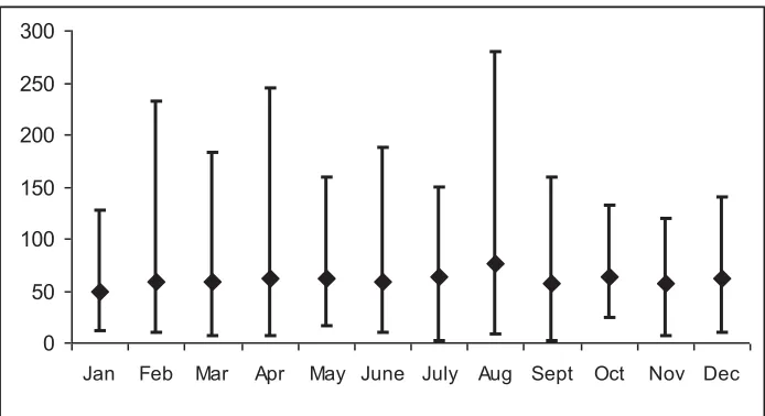
Figure 1.2: Mean and Range in Monthly Rainfall over 30 years at Hororata, Mid-Canterbury
from the NIWA Virtual Climate Station Network 2
Figure 3.1: Plots of model output () for cocksfoot growth rate compared to observed
growth data ({) from NZPBRA field experiments 19
Figure 3.2: A comparison between simulated () annual ryegrass yield and data ({)
from NZPBRA field experiment 20
Figure 3.3: Plots of model output () for lucerne growth rate compared to unpublished
growth data ({) from Smetham (1970) 20
Figure 3.4: Observed ({) and model predicted ()values for (A) kale, (B) forage rape,
and (C) pasja DM accumulation 22
Figure 3.5: Observed and predicted values for average LW for animals with data from Kitessa (1997) experiment II, utilising parameters from Oltjen et al.(2006)
(-U-) and parameters estimated in this study (); y=x 23
Figure 3.6: Observed (Sainz et al., 1995) and predicted values for EBW mass (A),
muscle (B), fat (C) and viscera (D); regression of y on x ; y=x 26 Figure 3.7: Comparison of simulated pasture covers ( ) for the grass- (A) and
legume-based (B) systems compared with data from the trial units (- -{- -)
for the production period 2007/08 to 2009/10 27
Figure 3.8: Comparison of simulated kale yield with observed data from the trial for
2008/09 (A) and 2009/10 (B) 29
Figure 4.1: Average annual pasture production for strategies 1 to 7 at 10 (■), 12 (i),
14 (▲), 16 (x) SU ha-1 34
Figure 4.2: Gross margins for strategies 1-7 at 10, 12, 14 and 16 SU ha-1 38
Figure 4.3: Expected returns (GM) vs Risk (SD of GM) for all strategies at 10, 12, 14
Definitions
Flushing: The practice of increasing the nutritional level of ewes prior to mating in order to increase ovulation rate.
Scanning Percentage, Scanning Rate: The results of ultra-sound scanning of pregnant ewes usually around two months prior to lambing in order to determine the number of foetuses carried by the ewe.
Stock Unit (SU): A measure of the carrying capacity of land or the feed requirement of stock; a standard stock unit is defined as a 55 kg ewe weaning a single lamb and equates to approximately 4200-4500 MJ ME year-1.
Terminal Sire: Rams, usually of a meat breed, mated to ewes to produce lambs destined for sale as meat rather than retained or sold as replacement stock.
Works: Slaughter facility, usually but not always, producing meat for export.
Acknowledgements
Summary
On the east coast of New Zealand, sheep and beef cattle are increasingly confined to dry hills and un-irrigated flat land as land suitable for irrigation is converted to other uses. Dryland farming is subject to significant variability in temperature and particularly rainfall between and within years with the most important climate risk being the point at which soils dry out and pasture production ceases in late spring/summer.
Improving pasture and animal performance and, in particular, the consistency of productivity and profitability in the face of a highly variable climate is complicated. The challenge is to utilise the 3-5 month window of opportunity for production between August and the end of the year to best advantage and without compromising the ability to feed ewes well in late summer/autumn prior to mating.
Key variables in this context are high lamb growth rates in order to finish as many lambs as possible before the risk of dry conditions becomes too high, and flexibility to respond to the growing conditions as they unfold.
The objectives of this research were to investigate, and demonstrate, opportunities for improving dryland sheep systems through increased lamb output, high pasture quality and utilisation, and flexibility to respond to climate and feed conditions.
The research included a farm scale trial, adaptation of an existing sheep farm simulation model LincFarm (Cacho et al.,1995; Finlayson et al., 1995) to replicate the trial situation, development of an algorithm for optimising de-stocking interventions in response to dry conditions, and evaluation of the long term implications on productivity, profitability and risk of a range of policy options using the model.
This report provides a summary of the field trials, and describes extensions to and evaluation of the LincFarm sheep systems model and its use to analyse a combination of stock and pasture options at different stocking rates based on the field trial. Development of the de-stocking algorithm and evaluation of a range of risk responses are presented elsewhere (Gicheha et al., 2013 a, b).
The field trials were based on two farm scale units at Lincoln University’s Silverwood Farm near
Hororata, a grass based unit of 87.8 ha and a legume based unit of 85.1 ha. The grass unit was stocked with a mixed age flock and trading cattle representing approximately 23 per cent of total stock units (SU) and the legume unit had the same mixed age ewe flock with additional older ewes
mated early as a ‘1stcycle mob’. Both were stocked at 14 SU ha-1 which is approximately 5 SU ha -1
higher than the regional monitor farm.
With the exception of poor performance on the legume unit in the first full year of the trial, results confirmed that it is possible to maintain high pasture quality and utilisation on a range of pasture types in dryland conditions with a high stocking rate and that this can lead to high scanning percentages and high pre- and post-weaning lamb growth rates.
quality and animal performance as well as building in flexibilities to respond to climate and pasture conditions when required can both increase returns per ha and reduce the variability of returns from one year to the next in comparison to the regional monitor farm.
These are un-replicated results from only two years of trial with one management policy on each unit. In order to investigate a broader range of climate conditions and management policies at different stocking rates, an analysis has been undertaken using the sheep farm simulation model LincFarm.
The LincFarm model was previously parametised for perennial ryegrass, white and red clovers, tall fescue and chicory, and for sheep. The model needed to be extended to include species used in the trial including annual ryegrass, cocksfoot, lucerne, both summer and winter brassicas and growing cattle.
Reparametisation of the mechanistic pasture model in Lincfarm for annual ryegrass, cocksfoot and lucerne, and development of a germination and emergence routine are described. Statistics of fit for the model against data sets from the NZ Plant Breeders Assoc. and unpublished data from Lincoln indicate coefficients of determination in excess of 0.95.
A simple model of dry matter accumulation of brassicas based on thermal time units and soil moisture is developed and provided similarly good fits to data on the growth of kale, forage rape and pasja (leaf turnip).
A model of beef growth and composition developed at Davis in the US (the Davis Growth Model, DGM; Oltjen et al., 1986) is reparametised for New Zealand conditions against data on growth of Angus x Hereford heifers at Lincoln. Statistics of fit are presented and were considered adequate for inclusion in LincFarm.
The extended model was then evaluated against data from the Silverwood trials and showed good
fits for total pasture cover, growth of lucerne and ‘switch’ pastures (perennial clovers oversown
with annual ryegrass), and drafting weights for cattle. Fits for the yield of kale were less good, especially in the first year of the trial when the yield of one kale variety in particular was very poor.
An analysis including 7 different combinations of stock and pasture mixes, each run at 4 stocking rates (SR = 10, 12, 14, 16 SU ha-1) over 19 years with the first 4 years discarded, using a soil moisture trigger value of 10% in the top 25 cm of soil (the same as in the Silverwood trial) was then conducted using LincFarm. Results include the mean and standard deviation (SD) or coefficient of variation (CV) for pasture production, lambing percent, carcass meat production and wool production per ha, and the income and variable costs (gross margin, GM) per ha.
Generally as SR increased so did the mean and CV of production and returns. A plot of the mean
GM against the SD of GM allows identification of the ‘risk efficient frontier’, those combinations
of strategy and SR which are dominant in terms of risk vs return. These include lower return-lower risk combinations, higher risk-higher returns combinations and those that are intermediate.
(ryegrass-white clover) at progressively higher stocking rates, suggesting that with these pasture types, high stocking rates are required to maintain pasture quality and obtain high returns.
Chapter 1
Introduction
Over the last decade, much of the irrigable land in the South Island of New Zealand has been converted to dairy and cropping. Even on dryland farms, dairy grazers have displaced sheep and beef stock units and as a consequence, sheep and beef cattle are increasingly being confined to dry hill country and some un-irrigated plains.
Dryland farming on the east coast of both main islands is subject to significant climate variability. Rainfall is the main climatic factor constraining pasture growth, with spring and summer rainfall accounting for 60 per cent of the variation in annual pasture production (Radcliffe & Baars, 1987). Baars & Waller (1979) identified both rainfall and temperature as influencing pasture production, with temperature playing an important role in pasture growth in winter and early spring.
On the Canterbury Plains, for example, winters are normally cool and wet and summers warm and dry - but not always so. Spring and autumn can either be wet or dry, warm or cool. A typical pattern of dryland pasture growth is shown in Figure 1.1. There is low growth during winter because soil temperatures are too low even though there may be sufficient moisture. Growth accelerates from mid-August as soil temperatures start to increase, reaching a peak around October/November followed by an abrupt drop in growth as soils dry out because of lack of rainfall in summer (any time from October onwards). A resurgence of growth may occur with autumn rains in April/May followed by a return to low growth again as temperatures drop from June onwards.
Figure 1.1: Three year average growth rate (July-June) of Ryegrass:White clover swards (kg DM ha
-1
day-1) at Hororata in Mid- Canterbury.
(Bywater et al., 2010)
However, spring growth may be delayed because of cooler or dryer conditions than are typical; spring/summer growth may cease early if there is little rainfall after September or it may continue throughout the season if there is a wet summer; there may or may not be autumn rain. There have been some years when there was no rain for 18 months; the 1988-89 drought for example is estimated to have cost farmers on the east coast of the North Island $240 million in reduced income and the total region $1000 million (Nield, 1990).
0 20 40 60 80
Although Figure 1.1 shows a typical pattern of growth, an analysis of 30 years of data from the NIWA virtual climate station network (Tait et al., 2006) for Hororata in mid Canterbury New Zealand (Latitude: -43.559962, Longitude: 171.84911) shows that in fact average monthly rainfall does not vary very much between months (Figure 1.2). However, the variability across years is extremely large, with the highest standard deviation and range in August and the lowest in October and November. In all months of the year, the range is greater than the mean.
Figure 1.2: Mean and Range in Monthly Rainfall over 30 years at Hororata, Mid-Canterbury from the NIWA Virtual Climate Station Network
Despite the climate patterns, Avery et al. (2008) suggest that pasture growth is reasonably reliable through winter and spring (the variability is less than the mean) until November but then becomes much less predictable (variability far exceeds the mean). The possibility of rainfall decreasing during late spring and summer to a point where grass growth ceases represents a major risk in dryland farming.
Seasonality in herbage production drives sheep production with ewes normally mated in autumn to match lambing with the spring pasture flush. Lambs are ready for slaughter any time throughout summer and autumn (Morris et al., 1993). As there is generally adequate high quality grass growth to support production from mid August through to sometime around November, this provides a
‘window of opportunity’ for production which is highly variable in length. Over late spring and
summer, farmers are in a high risk period when conditions can dry out quickly. Lambs which are not sold before then are at risk of growing much more slowly because of lower pasture availability and/or quality, extending the production period and requiring more feed in total. Variable rainfall patterns in late summer can make it difficult to provide adequate feed in situ to increase ewe live weights prior to mating to ensure high lambing percentages in the following season. If lambs are retained, grow slowly over summer, are held too long and start to compete with ewes for the best available feed, this may exacerbate the situation and jeopardise performance in the following year (Averyet al., 2008).
Improving pasture and animal performance in dryland farming systems is therefore complex because of the need to balance the nutritional requirement of different classes of livestock with a feed supply that fluctuates in quantity and quality within and between years (Finlayson et al., 1995). In most grazing sheep production enterprises, management interventions geared towards maximizing productivity and profitability generally target increased lamb growth rates, increased
0 50 100 150 200 250 300
stocking rate (SU ha-1) and/or increased lambing percentage (Diaz-Solis et al., 2006). However, increasing either of the latter two inevitably results in higher demand for feed and, where climate is a highly variable limiting factor, higher risk.
Walker (1995) and Diaz-Solis et al. (2003, 2006) suggest that setting stocking rate has been the dominant risk management decision in temperate grazing livestock systems. Traditionally, dryland livestock farmers in New Zealand have taken a conservative approach by keeping stocking rates
quite low, around 9 SU ha-1 in Canterbury/Marlborough (MAF, 2010). However, managing the
within and between season variability by short term manipulation of feed supply and/or animal feed requirement offers opportunities for improvements in such systems (Gray et al., 2008; Webby & Bywater, 2007).
The challenge is how best to utilise the 3-5 month window of opportunity for production described above to optimise productivity and profitability and to do so consistently from one year to the next despite highly variable rainfall patterns and without compromising the ability to feed ewes well in autumn. Key variables in this context are lamb growth rate in order to finish as many lambs as possible before the high risk period; and flexibility to respond quickly to the situation if and when condition become dry.
Several previous studies have shown that feed quality is a major determinant of both lamb growth rate and reproductive performance (Waghorn & Clark, 2004) and that use of alternative pasture species has the potential to improve the productivity and/or profitability of hill country (Grigg et al., 2008; Korte & Rhodes, 1993) and flatland farms (Fraser et al., 1999). Grigg et al. (2008) showed the advantage of managing for increased subterranean clover content on hill country, Avery et al. (2008) demonstrated the benefits of a high proportion of lucerne, and on dryland on the plains, Fraseret al. (1999) investigated use of a variety of high nutritive value species, including chicory and red clover. The downside of using these species is often limited feed supply over winter which can be addressed by including forage crops, forage cereals or annual ryegrass, but at a cost. Nevertheless, financial benefits of changing from a conventional feed supply system can be dramatic (Avery et al., 2008). Studies that placed emphasis on high feed quality, particularly before weaning, without using alternative pasture species are reported by Kinnell (1993) and Gray et al. (2008).
The objectives of this research were to investigate and demonstrate opportunities for improving dryland sheep systems by increasing productivity and profitability through increased lamb output with high pasture quality and utilisation, and by managing climatic variability by including flexibility to respond to climate and feed conditions as they develop. The study included a farm scale trial, development of an algorithm for optimising de-stocking and sales in light of prevailing conditions, adaptation of an existing sheep farm simulation model (LincFarm) to replicate the trial situation, and evaluation of the long term implications on productivity, profitability and risk of a range of policy options using the model.
Chapter 2
Field Trials
The field trial was carried out to investigate and demonstrate key aspects of high performance sheep systems in dryland environments. Key considerations were to develop feed supply systems on a farm scale that would deliver high feed quality throughout the growing season leading to high lamb growth rates, early sale of lambs and the opportunity to feed ewes well before mating to obtain high scanning rates the following year; and inclusion of flexible management strategies to allow rapid de-stocking as soon as conditions became dry to reduce variability of returns. Previous research has shown that risk (variability of returns) normally increases as returns (and stocking rates) increase (Cacho & Bywater, 1994; Hardaker et al., 1997).
In addition, the field trials were designed to investigate risk response indicators and provide base-line data for subsequent analysis of alternative policy options and risk responses using the simulation model, LincFarm. Details of the trial and its results are provided in Bywater et al. (2010, 2011 a, b); a summary is given here as background to the modelling.
2.1
Materials and methods
Two different approaches to maintaining high pasture quality and utilisation were investigated with non-replicated farm-scale trial units established at Hororata, mid-Canterbury: an intensively grazed conventional grass-based unit of 87.8 ha, and a high legume-content unit of 85.1 ha. Each unit had 16 paddocks, stocked at a target of 14 SU ha-1, which is 5 SU ha-1higher than the regional monitor farm (MAF, 2010). The first year of the trial in 2007/08 was used to bring data collection procedures and pasture and stock management into line with the trial protocol. Data collection was then carried out for two years, 2008/09 and 2009/10.
The grass unit included 13 paddocks of predominantly grass-based pasture (approximately 81 per cent of the unit); one paddock of lucerne (8 per cent of the unit); and two paddocks in a pasture-renewal rotation (11 per cent of the unit) including winter kale, followed by barley for silage and then a perennial grass mix in one paddock, and leaf turnip under-sown with a perennial grass mix in the other. Eight of the grass pastures were established ryegrass:clover pastures, two of which also contained cocksfoot and two tall fescue. Two older, brown top-dominant pastures were renewed through the above sequence in 2007/08 and two out of three Bareno brome pastures were renewed in 2008/09, all going into Alto ryegrass with white and red clover.
The underlying philosophy on this unit was that with a relatively high stocking rate, pasture utilisation would be high and pastures would be maintained in an actively growing state, ensuring a predominance of green leaf, minimum seed head development and a low proportion of dead material, and thus high feed quality (Litherland & Lambert, 2007).
On the legume unit there were four paddocks of predominantly grass-based pasture (30 per cent of
were renewed in 2007/08 and 2008/09 respectively, also going into the Alto ryegrass:clover mix. The five switch pastures were established at the start of the trial in 2007. In 2009/10, pastures on this unit changed to five paddocks of grass-based pasture and four paddocks of lucerne through the renewal programme.
The philosophy on this unit was that legumes provide high nutritive value feeds and retain their quality for longer than grasses if left un-grazed (Hyslop et al., 2000) so that control of pastures is less critical. Forage rape was included in the renewal sequence to provide flushing feed for ewes at a time when switch pastures had recently been over-drilled with annual ryegrass and were unavailable for grazing.
Stock included a mixed age flock and 18 month-old trading cattle (23 per cent of total SU) on the grass unit and a mixed aged flock with additional older ewes on the legume unit. The main sheep
breed was Coopworths from Lincoln University’s Ashley Dene breeding flock (Nsoso et al., 1999), mated to terminal sires.
With a high stocking rate to maintain pasture quality, the risks and consequences of running out of feed when conditions become dry are high, making it more important to build in flexibilities to reduce stocking rate quickly when required. Cattle were purchased in May and sold any time after October according to feed conditions. Older ewes were lambed on 20 August (grass unit) or 13
August (legume unit), 3 and 4 weeks before the main mob respectively (‘1stcycle’ ewes), allowing
early weaning, sale of lambs and culling of ewes if required (7 per cent and 20 per cent of SU on the grass and legume units, respectively). Main mob ewes were lambed on 6 September on both units with lambs weaned at 25 kg, or earlier if conditions became dry. Ewes were set stocked on individual paddocks one week before the start of lambing until weaning except for ewes on switch pastures. Pasture mass had diminished quickly following set stocking of these pastures in 2007/08 so they were subsequently rotationally grazed from before lambing to weaning. Store lambs were sold at weaning based on projected feed availability at the time. The lucerne and leaf turnip paddocks on the grass unit and two lucerne paddocks on the legume unit were targeted for lamb finishing, but were also available for ewes if required. Home grown or purchased silage or balage was used as a last resort to fill feed supply deficits.
Soil moisture readings were taken at weekly intervals from August to December and at fortnightly intervals for the rest of the year to 25, 50, and 75 cm soil depth in three paddocks on each trial unit. Pasture cover was assessed on all paddocks on the same schedule using a plate meter calibrated to the different pasture types every three months. Four grazing exclusion cages were placed in each of 12 paddocks, two each of the main pasture types. Two cages in each of these paddocks were cut every two weeks to 2 cm to estimate pasture growth rates giving a 28 day cutting interval for each cage. Pasture samples were taken from the same paddocks at 6 weekly intervals, cut to 2 cm and sub-sampled for herbage quality analysis using near infrared spectroscopy and dissection into botanical species components.
pregnancy rank in June. Further details of measurements and management are provided in Bywater et al. (2010).
Variables initially investigated as indicators of the need to de-stock were soil moisture, pasture growth rate, and average farm cover. To be effective, de-stocking decisions need to be implemented quickly, allowing for any marketing delays which are usually 7-10 days, so as to pre-empt market responses to dry conditions, such as difficulty in obtaining space at the meat works and reduced price of store stock (Gicheha, 2011). Under the fortnightly pasture sampling regime in this trial, pasture growth rate information was not available soon enough to be useful. Also, pasture covers did not vary sufficiently to serve as a meaningful indicator. On the other hand, soil
moisture levels to 25 cm depth (SML25) were read and available weekly and provided a clear
indication of changes in growing conditions. A value of 10 per cent SML25 was used as the trigger to begin de-stocking as this approximates the point at which grass growth stops (N. Smith, Lincoln University, pers. comm., 2007). A de-stocking priority list was defined for each unit, depending on sales to date and whether weaning had occurred. Trading cattle and cull ewes were generally sold first, followed by store lambs, prime lambs, and then capital stock.
2.2
Results
Results of the trial are summarised below and are presented in greater detail in Bywater et al.(2010, 2011 a, b).
There was no difference between the two units in total annual pasture production calculated as a rolling three-period average over three years. Production was 10,414 kg DM ha-1year-1 on the grass unit and 10,336 kg DM ha-1year-1 on the legume unit. With the high stocking rate, pasture cover was maintained at a relatively low level and did not vary much during the year, despite large variations in pasture growth rate and animal demand. Farm cover averaged 982.9 kg DM ha-1 ± 219.2 kg DM ha-1 (standard deviation) on the grass unit and 1193.9 ± 250.8 kg DM ha-1 on the legume unit over the last two years of the trial.
The low pasture covers suggest that there was a good balance between feed supply and demand and that pasture utilisation was high. Based on the annual average pasture growth during the trial described above, and the total feed requirement of stock calculated from stock numbers and average performance recorded over the last two years of the trial using standard equations (AFRC, 1993), average pasture utilisation was estimated to be 71.7 per cent on the grass unit and 74.3 per cent on the legume unit.
The balance between feed demand and supply was close on the grass unit except in peak growth periods in spring and autumn but on the legume unit, there was a feed supply deficit in December and another in March (Bywater et al., 2011 a). The deficit in December could be relatively easily managed through stock sales, one of the response variables included in the trial. The March deficit
was less easy to manage. This arose because ‘switch’ pastures on the legume unit were oversown
with annual ryegrass in February/March and were therefore not available for grazing at this time; and because the legume unit was stocked entirely with sheep which increased feed demand for flushing in March compared with the grass unit where nearly a quarter of the SU were cattle, sold earlier in the season.
shown in Table 2.1. In 2008/09, ME averaged 11.6 and 11.5 MJ/kg DM on the grass and legume units respectively from April to October and then dropped when conditions became dry. Climate conditions in 2008/09 were such that soil moisture levels dropped to around 10 per cent by volume in the first week in November and did not increase again until February. In contrast, soil moisture levels remained above 20 per cent throughout the 2009/10 season. This is reflected in the pasture quality with average ME levels from April to the last reading in January of 11.6 and 11.4 MJ/kg DM on the grass and legume units, respectively. None of these differences were significant.
Table 2.1: Average pasture quality (MJ ME/kg DM) on the grass and legume units in 2008/09 and 2009/10
2008/09 17/04 12/05 11/06 7/07 4/08 16/09 31/10 8/12 19/01
Grass 11.4 11.8 12.3 11.4 11.5 11.2 11.4 10.0 10.1
Legume 11.1 11.4 12.1 11.4 11.7 11.8 11.3 9.3 10.4
2009/10 3/03 14/04 11/06 7/07 4/08 28/09 31/10 18/11 26/01
Grass 10.5 11.7 12.3 11.2 11.6 11.3 11.6 11.6 11.1
Legume 10.7 11.9 12.1 11.6 11.9 11.3 11.5 12.0 9.1
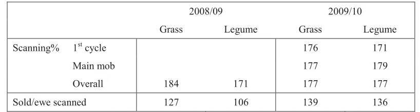
With pasture quality at or close to target, animal performance was also close to or above target. Targets for reproduction performance were to achieve 175 per cent scanning and 145 per cent sale. Scanning percentages were close to or above target on both units but survival-to-sale was not (Table 2.2). Death rates of both ewes and lambs were higher than expected. Ewe deaths were 6.4 per cent and 8.1 per cent in 2008/09 and 7.3 per cent and 6.5 per cent in 2009/10 on the grass and legume units, respectively. Lamb losses between scanning and sale were very high, particularly on the legume unit in 2008/09. Bad weather in late August 2008 caused a number of ewe and lamb deaths, and a confirmed outbreak of Salmonella Brandenburg on both units in 2009/10 contributed to the high losses but may not be sufficient to explain them completely. Nevertheless, the losses resulted in lower than expected lamb sales particularly on the legume unit in 2008/09.
Table 2.2: Lambing percentage at scanning and survival to sale on the grass and legume units in 2008/09 and 2009/10
2008/09 2009/10
Grass Legume Grass Legume
Scanning% 1stcycle 176 171
Main mob 177 179
Overall 184 171 177 177
Sold/ewe scanned 127 106 139 136
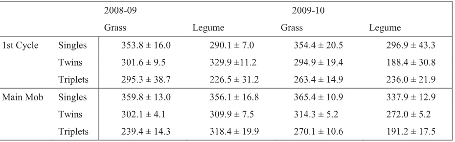
Pre-weaning growth rates of single and twin lambs (Table 2.3) compare well with those observed in previous studies at high stocking rates on dryland (Ates et al., 2006, 2008). They are much
higher than the average pre-weaning growth rate of 221 g day-1 on 15 summer-dry farms
model (Gilmore et al., 2009) shows an overall mean and standard error of 304 r 12 g day-1. While there were significant differences due to litter size (singles, twins and triplets P<0.001), mob (first cycle and main mob, P<0.05), and year (P<0.01), there was no difference between the two units.
Post-weaning growth rate data were also available on 120 lambs. However, stock disposal policies at weaning included sale of lambs which had reached drafting weight and sale as stores of those which could not be finished on the assessed pasture available at that time. In other words the largest and smallest animals are not included in the post-weaning data which therefore should be
treated with some caution. Average post-weaning growth rate was 139 r 32 g day-1 with
significant differences attributable to litter size, mob and year. Again this is much higher than the average post-weaning growth rate on summer-dry farms of 75 g day-1found by Everest and Scales (1983).
Table 2.3: Mean and standard error of pre-weaning growth rates of lambs on the grass and legume units in 2008/09 and 2009/10
2008-09 2009-10
Grass Legume Grass Legume
1st Cycle Singles 353.8 ± 16.0 290.1 ± 7.0 354.4 ± 20.5 296.9 ± 43.3
Twins 301.6 ± 9.5 329.9 ±11.2 294.9 ± 19.4 188.4 ± 30.8
Triplets 295.3 ± 38.7 226.5 ± 31.2 263.4 ± 14.9 236.0 ± 21.9
Main Mob Singles 359.8 ± 13.0 356.1 ± 16.8 365.4 ± 10.9 337.9 ± 12.9
Twins 302.1 ± 4.1 309.9 ± 7.5 314.3 ± 5.2 272.0 ± 5.2
Triplets 239.4 ± 14.3 318.4 ± 19.9 270.1 ± 10.6 191.2 ± 17.5
Taking both pre-and post-weaning growth rates into account, average lamb growth rates from birth to sale over both years and both units was 295 r 3 g day-1, slightly lower than the target of 300 g day-1.
In summary, the trial confirmed that it is possible to maintain high pasture quality on a range of pasture types including conventional ryegrass:clover pastures with a high stocking rate on dryland farms, and that this will lead to high scanning percentages and high pre-and post-weaning lamb growth rates.
2.3
Climate-risk responses
As noted, SML25 dropped to 10 per cent in the first week of November 2008 which triggered the decision to begin de-stocking as rapidly as possible subject to availability of killing space. Weaning of both first cycle and main mob lambs was completed before the end of the month with drafts of lambs and first cycle cull ewes going to the export works. All cattle were sold by 24 November. The remaining feed supply was assessed and light lambs which could not be finished were sold store in early December and any remaining cull ewes were sold over December and January as space became available.
weaning the first cycle mob at the end of November; main mob lambs were weaned on 3 and 12 December on the grass and legume units respectively, with cattle sold in January, cull ewes in February, and lambs sales through to mid-March.
Because of the rainfall patterns in 2008/09, pasture growth rates decreased early and a high proportion of lambs were sold as stores. At weaning in 2008 there was little feed available on the legume unit in particular, primarily because of very poor performance of the lucerne paddocks which were old pastures. This resulted in a much higher proportion of lambs being sold early as stores on the legume compared to the grass unit; only 26.5 per cent and 68.0 per cent of lambs from the legume and grass units, respectively, were sold to the export market in 2008/09 whereas in 2009/10, 73.8 per cent and 76.0 per cent went to the export meat works from these units. Thus, the high lamb wastage rate in 2008/09 was compounded by poor finishing on the legume unit.
The dry conditions lasted until February 2009 and had the potential to cause a significant feed deficit that could have restricted ewe intake prior to mating, potentially leading to a lower lambing percentage in the following season. The flexibility and risk management responses on both units worked well in this situation with essentially all stock sales completed within three-and-a-half weeks of reaching the trigger point of 10 per cent SML25 (except for some cull ewes which took longer to move off farm). Both came through the dry spell with no real difference in pasture covers between the two years – in fact covers between November and February on the legume unit were slightly higher in 2008/09. Also pregnancy scanning percentages were similar in both years (Table 2.2). Unfortunately because of the high lamb wastage and failure of the lucerne on the legume unit, this did not translate into high production and profitability for the season on that unit. 2009/10 was a much more favourable season and all stock were held on both trial units for longer.
The main objective of risk management responses is to reduce the variability in performance and profit between years by maximising performance in good years and minimising losses in poor years. Selected financial performance indicators for the two units in 2008/09 and 2009/10 from
Bywater et al. (2011 a) are shown in Table 2.4 compared with the Canterbury/Marlborough
Table 2.4: Comparison of key financial indicators on the grass and legume units with the Canterbury/
Marlborough Monitor Farm (MAF, 2010) from Bywater et al.(2011 a)
Grass Unit Legume Unit MAF Monitor Farm
Effective area (ha) 87.8 85.1 469
2008-09 2009-10 Diff % 2008-09 2009-10 Diff % 2008-09 2009-10 Diff %
Total Stock units 1231 1172 -4.8 1205 1223 1.5 4096 4125 0.7
SU ha-1 14.0 13.3 -4.8 13.7 13.9 1.5 8.7 8.8 0.7
Lambing % to sale 126.5 139.3 10.1 105.9 136.0 28.4 125.0 138.0 10.4
$ $ $ $ $ $
Net Income1 ha-1
SU-1 1,211 86.34 1,170 87.65 -3.3 1.5 898 63.42 1083 75.39 20.7 18.9 866 99.13 965 109.77 11.5 10.7
Direct Costs2 ha-1
SU-1 351 25.07 357 26.74 1.6 6.7 492 34.74 481 33.51 -2.1 -3.5 375 46.80 436 49.56 16.2 5.9
Gross Margin ha-1
SU-1 859 61.27 813 60.91 -5.4 -0.6 406 28.68 602 41.88 48.2 46.0 491 52.32 530 60.20 7.9 15.1
Overheads3 ha-1 72 61 -14.7 72 61 -14.7 80 72.44 -9.1
Surplus4 ha-1
SU-1 787 55.51 752 56.33 -4.5 1.5 334 23.62 541 37.62 61.7 59.3 411 42.38 457 51.97 11.2 22.6 1
Includes sale of culls and wool and cost of replacements
2
Does not include labour
3
Farm overheads pro-rated ha-1 for the grass and legume units; does not include interest costs
4
Does not include labour, wages of management or interest charges
The difference between years in all financial indicators except for overhead charges is much smaller on the grass unit than on the monitor farm, suggesting that the ability to respond rapidly to varying growing conditions has the potential to reduce year to year variability in farm financial results, i.e. reduce risk. The same is not true of the legume unit where poor performance in 2008/09 resulted in a much larger difference between years simply because problems encountered during that season were not repeated the following year. This reinforces the importance of being able to finish lambs quickly in this environment, making it easier to deal with dry conditions if and when they arise.
Chapter 3
The LincFarm Model
To investigate a range of pasture and stock policy combinations over a range of climate situations, a simulation analysis has been undertaken using the sheep farm simulation model, LincFarm (Cacho et al., 1995; Finlayson et al., 1995). This has been combined with a de-stocking and marketing algorithm developed by Gicheha et al. (2013 a) to simulate tactical interventions in response to changes in climatic conditions and feed supply in dryland grazing systems.
LincFarm is designed to evaluate alternative strategies for managing pastoral sheep systems. It has the facility to subdivide the farm into paddocks, allocated to blocks, in which different animal, pasture and management parameters can be applied. Animals are grouped into mobs, each with different management. It has the capacity to run an analysis for as many years as suitable weather data are available, with the state of the system carried forward from one year to the next.
LincFarm includes a mechanistic animal model described in Finlayson et al. (1995), a plant model
described in Bywater et al. (1999), and a calendar of management events which schedules
interventions such as purchases and sales, mating, shearing, drafting, etc and which controls the operation of the animals/mobs and paddocks/blocks (Cacho et al., 1995). The management calendar includes a limited number of conditional decisions, meaning that decisions made at a particular point in time in the simulation can be conditional on the situation existing at that time rather than being fixed at the start of the simulation. For example, hay making can be conditional on current pasture mass and hay feeding can be conditional on the condition of the animals. While the extent of conditional decision making needed to be expanded to include tactical marketing and destocking interventions in response to climatic variability, the fact that this is possible is essential for the analysis to be undertaken.
LincFarm has both front- and back-end programmes used to prepare input files and produce output reports respectively. Input data files define the farm, pasture and animal parameters, management, and experimental treatments to be simulated. There is flexibility to determine the output from the model, which allows a detailed analysis of the reasons behind an improved enterprise performance where required.
Prior to the analysis reported here, the model was parameterised for perennial ryegrass, white and red clovers, tall fescue and chicory, and for sheep. In the trial, pasture and stock types included annual ryegrass, cocksfoot, lucerne, both summer and winter forage Brassicas, and growing cattle. Thus there was a need to extend LincFarm to parameterise the pasture model for three additional pasture species, incorporate a crop model for Brassicas, and include a model of beef growth and composition. Following their inclusion, the revised LincFarm model was then evaluated against data obtained from the trial (Bywater et al., 2010).
3.1
Setting parameters of a mechanistic pasture growth model
photosynthesis over time and depth in the canopy. The model is separated into five growth sub-models (photosynthesis, growth, reproduction, specific leaf area and assimilate partitioning), two site dependent sub-models (radiation and soil moisture) which are run once per day per site and two site and growth interaction sub-models (water stress and light capture).
The model is specified in two forms, one which represents the above ground canopy and is used for grasses and some clovers (Bywater et al., 1999) and one which includes a root component used for some legumes and herbs such as red clover and chicory (Bywater et al., 2000). Annual ryegrass and cocksfoot were specified using the first version of the model representing above ground components only and requiring a total of 45 parameters, while the second version including the root sub-model was used for lucerne requiring an additional 9 parameters.
Peri et al. (2005) suggest that in related species such as grasses, differences in parameters controlling response to the main environmental variables, rather than the entire parameter set describing the plant, influence net leaf photosynthesis and subsequent productivity in plant growth
simulation models. For annual ryegrass and cocksfoot in ambient [CO]2 conditions, the main
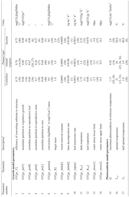
15 Table 3.1 : P a ra m e te rs e sti mat e s for co cks foot, annu a l ry egra ss and luce rne p astur es for the can opy gr o w th mod e l aram eter mb er P aram eter Description 1 P astu re t y pe 1 Unit s C o ck sf oot An n u al ry e g ras s lu cern e G r o w th m o del para m e ter s GV[g v _ Y] ef ficienc y of co n v erti n g s u bstr
ate to stru
cture 0.75 (39) 0.76 (14,3 9 ) 0.75 (40) mg[ C O2 ](kg D M h a -1 ) -1 GV[g v _pieV] assi m ilate partition to v egeta ti v e g ro w th 0.60 (16) 0.60 (27) 0.88 (8) m g [C O 2 ]m -2 GV[g v _pie R ] assi m ilate partition to rep rodu ctiv e lea f 0.66 (38) 0.67 (20, 27) 0.88 (8) s GV[g v _pieS] assi m ilate partition to rep rodu ctiv e ste m 0.3 (38) 0.26 (27) 0.27 (6) s GV[g v _pie L ] assi m ilate partition to root 0.68 (40) 0.68 (40) 0.60 (5) s G V [gv_ ga mma ] co nve rs io n ( k gD M ha -1 to m g CO 2 m
-2 ) m
a ss 161 (39) 161 (39) 161 (39) mg[ C O2 ](kg D M h a -1 ) -1 GV[g v _ R] targ et m a ss 1.0 1.0 2.0 (33) GV[g v _deltaE] w o rm re m o v al co nsta n t 0.000 5 (38) 0.000 5 (38) 0.000 5 (38) GV[g v _deltaD] base decom positio n rate 0.014 8 (1) 0.014 8 (1) 0.014 8 (1) kg ha -1 d -1 GV[g v _ sigm a] leaf se n esce n ce rate 0.001 1 (39) 0.001 2 (18) 0.001 1 (39) kg ha -1 d -1 GV[g v _ Rm1 ] dark respiration 1.72 (1) 1.6 (22) 4.32 (33) m g [C O2 ]g -1 h -1 GV[g v _ Rm2 ] leaf respiration 0.08 (1) 0.061 (14) 0.078 (1) mg[ C O2 ]g -1 h -1 GV[g v _ stress1] w ater stre ss lo w er li m it -2 .2 (10) -2 .5 (7) -3 .8 (37) Mp a GV[g v _ stress2] w ater stre ss u pper li m it -0 .2 -0 .5 -0 .2 Mp a Photosynthesis m o del para m e ter s Q m ax im u m ph otos y n th e
sis at re
fe rence te m p erature 1.17 (29, 38) 0.82 (14) 2.0 (38) mg[ C O2 ]m – 2 (leaf) s -1 Tref optim a l te m p erat u re 21 (13, 32) 20
(23, 26, 36)
16 Table 3 .1 : Co ntd ’ P aram eter nu mb er P aram eter Description 1 P astu re t y pe 1 Unit s C o ck sf oot An n u al ry e g ras s lu cern e 18 Al p h a peak leaf ph otos y n th e sis e ff ici enc y 0.01 (15) 0.076 (19) 0.022 (32) mg[ C O2 ]J -1-19 T h eta cu rv at u re para m eter in lea f photos y n th e sis respons e 0.81 (38) 0.86 (15) 0.61 (32) Di m e n sio n les s Repro duction m o del para m e ters 20 A m in im u m s u stain ab le S L A 0.007 5 (1) 0.04 (30) 0.092 (11) m -2 (lea f) m 2 21 B dif fere n ce bet w een A a n d SLA w h e n g ro w n i n t h e dark -0 .001 (1) -0 .078 (1) -. 0017 (11) s 22 C in sta n ta n eo u
s rate of
cha n g e o f S L A 0.166 1 (1) 0.165 (20) 0.0 (11) s 23 M rate of ste m m at u ration 0.09 (38) 0.09 (38) 0.0 (32) Mg[CO 2 ]m -2 d -1 24 Flg fl a g leaf fr action o f th
e total re
produ ctiv e leaf 0.21 (1) 0.21 (1) 0.0 (32) 25 t1 day w h e n ste m elo ng atio n star t 273 (24) 282 (16) 320 (14) day s 26 t2 day w h e n ste m m aturatio n star ts – day o f ear e m er ge nc e 306 (24) 296 (16) 90 (14) day s 27 t3 day w h e n ste m se n esce n ce sta rts 324 (24) 315 (16) 90 (14) day s 28 t4 day w h e n ste m elo ng atio n ceases 333 (24) 324 (16) 75 (14) day s Light ca pture m o del para m e ters 29 K exti n ction co e ff ic ient 0.44 (12) 0.63 (21, 27) 1.03 (34) m -2 (g roun d) m 2 (leaf) 30 Kv exti n ction co e ff ic ient v e g etati v e leaf 0.88 (37) 0.88 (37) 0.94 (10) s 31 Kr exti n ction co e ff ic ient rep rodu ctiv e lea f 0.92 (37) 0.92 (37) 0.94 (10) s 32 Km exti n ction co e ff ic ient rep rodu ctiv e ste m 0.92 (37) 0.92 (37) 0.94 (10) s 33 Epsilon rep rodu ctiv
e leaf eleva
17 : C o ntd’ aram eter mb er P aram eter Description 1 P astu re t y pe 1 Unit s C o ck sf oot An n u al ry e g ras s lu cern e cm ligh t cap tu re eff icie n c y of m at u re ste m 0.003 (15) 0.003 (15) 0.003 (15) ha k gD M -1 cd ligh t cap tu re eff icie n c y of lea f, sh eat h and dead m ater ial 0.009 (15) 0.009 (15) 0.009 (15) s cmr ligh t cap tu re eff icie n c y of rep rodu ctiv e ste m a n d leaf 0.000 46 (15) 0.000 46 (15) 0.000 36 (15) s wd prop ortion of dead m ater ial i n m ix ed la y er 0.28 (33) 0.28 (33) ) 0.28 (33, 39) kg D M ha -1 Specific lea f area m o del par a m e ters mi nS L A
leaf area ratio of
v ege tati v e g reen 0.001 9 (37) 0.001 86 (211) 0.001 9 (33) h
a (leaf) kg
The process of estimating parameter values for simulating lucerne growth followed that for annual ryegrass and cocksfoot. Sensitivity analysis of the model parameters showed a similar pattern to the grasses. Where values were not available for lucerne specifically, those from pasture species with similar growth characteristics were obtained. In addition to the parameters presented in Table 3.1, the lucerne model utilises the root component which requires an extra 9 parameters shown in Table 3.2. The root model is important in modelling lucerne growth and productivity in situations where photosynthesis exceeds the requirements for carbon, as the excess carbohydrates are stored in the taproot and crown, mainly in the form of starch (McAdam & Nelson, 2003).
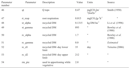
Table 3.2: Lucerne root growth model parameters
A sensitivity analysis was also carried out for the root model parameters and, with the exception of the parameter describing recycled dry matter (rc_alpha), they were shown not to significantly affect the TDM, GDM and LM components.
LincFarm has not previously included a germination routine so in order to simulate growth of annual pasture species, a germination procedure has been developed. Temperature (expressed as thermal time requirements for germination and emergence) and rainfall are required for seeds to germinate and emerge. The model simply accumulates thermal time (Tt), also known as heat units or growing degree days, and rainfall after the sowing date and once the threshold values are reached, the crop is assumed to be established. Estimated germination and emergence thermal time (Tt) requirements for annual ryegrass are 90 and 145 degree-days (oCd) respectively (Moot et al., 2000). Rainfall of 10.0-13.0 mm after 1st of March (Cocks & Donald, 1973; Gramshaw & Stern, 1977) has been shown to cause germination and subsequent emergence.
Germination is considered to occur when the shoot reaches 1.0 mm in length. Hill et al. (1985) obtained a dry weight per tiller and leaf after germination of 0.15 and 0.03 grams respectively, a number of leaves per tiller of 3.2 and a total number of tillers of 25 at day 35 after sowing. This
Parameter number
Parameter Description Value Units Source
46 qt Q tops 0.47 mg[CO2]m–
2
(leaf)s-1
Smith (1950)
47 rt_resp root respiration 0.015 mg[CO2]g-1h-1 "
48 st_alpha recycled DM 0.1315 kg DM ha-1 Li et al. (1996)
49 st_gamma recycled DM 895 " Bowley et al.
(1988)
50 rc_alpha recycled DM 1.7 " Bowley et al.
(1988)
51 rc_gamma recycled DM 0.0 " Estimated
52 rc_d1 recycled DM–day lower
limit
35 day Teixeira (2006)
53 rc_d2 recycled DM–day upper
limit
212 " "
54 rm_pie used in apportioning while
vegetative
information, together with a seed sowing rate of 18.0-25.0 kg ha-1 (Agricom, 2010), estimates of 100,000 seeds of annual ryegrass per kilogram seed, and a 90.0 per cent germination rate (Hill et al., 1985), was used to estimate an initial mass of annual ryegrass at germination of 22.14 kg DM ha-1.With inclusion of the germination procedure in LincFarm and specification of parameter values described in Table 3.1, the model was evaluated against data for cocksfoot and annual ryegrass (six data-sets for each pasture type) provided by the New Zealand Plant Breeders Research Association (L.Dick, NZPBRA, pers. com., 1999) and unpublished data on lucerne growth at Lincoln, New Zealand from Smetham (1970). Plots of model estimates against the data are shown in Figures 3.1 – 3.3 and statistics of fit using methods described by Kobayashi & Us Salam (2000) are given in Table 3.3.
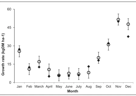
Estimated growth rates of cocksfoot against NZPBRA field data are shown in Figure 3.1. Modelled pasture growth rates for cocksfoot were generally within one standard deviation of the mean field data except for a period around April and December when it fell below the data and in a period after August when it slightly overestimate growth rate.
Figure 3.1: Plots of model output () for cocksfoot growth rate compared to observed growth data
({) from NZPBRA field experiments
Figure 3.2 shows model estimates of annual ryegrass yield against measured growth data over two years from NZPBRA. Model values match the field data except for some data points around October 1995 and May 1996 which fell outside one standard deviation of the mean values. The pattern of change in growth rate with season closely mirrored that observed in the trials. Annual ryegrass is assumed to die approximately 14 days after flowering which explains its sharp decline after November following flowering.
0 15 30 45 60
Jan Feb March April May June July Aug Sep Oct Nov Dec
Grow
th rate
(kgDM
ha-1)
Figure 3.2: A comparison between simulated () annual ryegrass yield and data ({) from NZPBRA field experiment
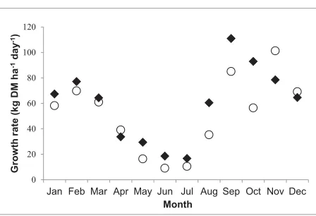
Figure 3.3 shows plots of model output and unpublished data on growth rates of pure lucerne grown at Lincoln from Smetham (1970). Generally, the modelled growth rates were within one standard deviation of the field data with the exception of a period around May and another around August - October when the model tended to overestimate the growth rate.
Figure 3.3: Plots of model output () for lucerne growth rate compared to unpublished growth data
({) from Smetham (1970)
In all other instances, the model prediction fell within one standard deviation, suggesting that the model parameters obtained from the literature search are sufficient to simulate lucerne growth and productivity in this environment.
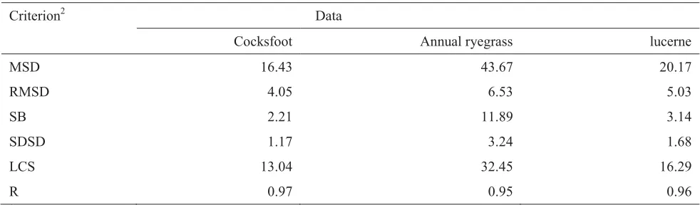
Table 3.3 presents a summary of statistics for the pasture model evaluation. Statistical methods from Kobayashi & Us Salam (2000) include the mean squared deviation (MSD) and root mean squared deviation (RMSD) which indicate the overall deviation of the model output from the measured value. MSD is then partitioned into components which represent different aspects of the deviation. The squared deviation or SB measures the difference between the means of the predicted and observed values. The difference between the standard deviations of the predicted and observed values (SDSD) indicates the extent to which the model fails to simulate the magnitude of fluctuation among the nobservations, and the lack of positive correlation weighted by the standard deviations (LCS) shows the extent to which the model fails to simulate the pattern of fluctuations across the nmeasurements.
0 500 1000 1500 2000 2500 3000 3500
Apr-95 Jul-95 Oct-95 Feb-96 May-96 Aug-96 Dec-96
Y
ield
(kgDM
ha
-1)
Time
0 20 40 60 80 100 120
Jan Feb Mar Apr May Jun Jul Aug Sep Oct Nov Dec
Grow
th
rate (kg DM ha
-1
day
-1)
Table 3.3: Statistics for the set of pasture model parameters1used in simulating yield (kg ha-1) of cocksfoot, annual ryegrass and lucerne
Criterion2 Data
Cocksfoot Annual ryegrass lucerne
MSD 16.43 43.67 20.17
RMSD 4.05 6.53 5.03
SB 2.21 11.89 3.14
SDSD 1.17 3.24 1.68
LCS 13.04 32.45 16.29
R 0.97 0.95 0.96
1
See Tables 3.1 and 3.2 for the parameters
2
See text for description of the evaluation criteria
In general the RMSD in kg ha-1 is quite low which is reflected in the high values of the correlation coefficients for all three species indicating that only small differences exist between model output and measured values. In all cases, LCS which relates to the pattern of fluctuations across the measurements, is the major component contributing to MSD. For instance for cocksfoot, it contributed 79.37 per cent of the MSD while SB, which measures the difference between the means of the predicted and observed values, only contributed 12.90 per cent. SDSD, which reflects the ability to simulate the magnitude of fluctuations among the observations, is very small in all cases.
3.2
Development of a simple crop model for brassicas
Thermal time (Tt) has been proposed to describe the phenological development of plants as an alternative to calendar days in projecting crop yield (Morrison et al., 1989). Various studies have established a linear relationship between number of leaves per stem and accumulated temperature (oCd) in wheat (Gallagher, 1979), corn (Zea mays L.) (Warrington & Kanemasu, 1983), summer rape (Morrison & McVetty, 1991), Pasja or leaf turnip (Brassica campestris x napus) (Nanda et al., 1995), and kale (Wilson et al., 2004). Adams et al. (2005) observed that yield of brassicas (Goliath rape, Green Globe turnip, Gruner kale and Kestrel kale) was linear in relation to Tt. Chakwizira (2008) identified a strong linear relationship (R2=0.99) between dry matter accumulation and Tt for kale and Pasja, with and without phosphate fertiliser application, of 800.0 and 420 kg DM ha-1 for every 100.0 oCd respectively (mean of all P fertiliser treatments) with a base temperature of 0.0 oC (Mootet al. 2007). Adams et al. (2005) obtained a value of 667 kg DM ha-1for every 100.0 oCd for rape with a base temperature of 4.0 oC. Though other production factors such as soil fertility, pest and diseases affect forage crop dry matter accumulation, most often the main yield limiting factor is soil water (Wilson et al., 2006). Hence soil moisture has been included as a modifier in an equation for estimating the dry matter accumulation of Brassicas:
DM = DMAccumulationPer0Cd x Tt x MoistureModifyer
Where DMAccumaltionPer0Cd represents the amount of dry matter accumulated per oCd and
data from Chakwizira (2008) and Adams et al. (2005) shows that, the modelled dry matter for these forage crops fell within one standard deviation of experimental values (Figure 3.4).
Pasja differs from kale and rape in that it has a crown, usually at or below ground level, from which leaves grow, enabling leaf regeneration after defoliation. Input variables for the model allow the user to define the minimum pasture cover (in per cent) below which no crop re-growth occurs following grazing. Setting the value to zero means a crop that has been grazed down and has a potential to re-grow, as is the case with Pasja, does not die. Chakwizira (2008) established that the high leaf to stem ratio obtained for Pasja indicated that its dry matter was essentially made up of leaf with the crown constituting less than 6.0 per cent of dry matter (48.0 g m-2). This is similar to the value of approximately 8.0 per cent reported by Wilson et al. (2006). Thus, since growth 1 occurs from the crown, dry matter accumulation for Pasja does not start at zero.
Figure 3.4: Observed ({{) and model predicted ()values for (A) kale, (B) forage rape, and (C) pasja
DM accumulation
3.3
Beef growth and composition model
The third extension to LincFarm required for the analysis is inclusion of a beef cattle growth model. Oltjen et al. (1986) described a dynamic model of post-weaning growth and composition in beef cattle (Davis Growth Model; DGM) based on fundamental biological concepts of hyperplasia and hypertrophy, earlier developed by Baldwin & Black (1979) and Burleigh (1980), but applied at the whole animal level. The DGM was chosen to simulate growth and composition of young cattle under New Zealand grazing conditions because it explicitly represents factors such as the animal’s
genetic background and nutritional history which are important determinants of performance when extended to new situations (Oltjen et al., 1985; Sainz et al., 1995).
0 4000 8000 12000 16000
0 500 1000 1500 2000
DM
(
k
g ha
-1)
A
0 4000 8000 12000
0 500 1000 1500 2000
DM (kg ha
-1)
B
0 4000 8000
0 500 1000 1500 2000
DM
(
k
g ha
-1)
The DGM was originally parameterised using individual data from Garrett (1980) and Byers & Moffitt (1979) for medium-framed British steers. Utilising data from Brazilian Nellore cattle, Sainz et al. (2006) found that the original model under-predicted final empty body mass, body fat and energy and that it was necessary to use revised model parameters to account for a higher efficiency of energy utilisation in the Nellore animals. This observation emphasises the potential importance of estimating breed specific parameters for the model when applying it to different production systems.
In the New Zealand study of Kitessa (1997), two experiments were carried out to investigate the influence of co-grazing sheep and cattle on cattle liveweight (LW) and liveweight gain (LWG) under continuous or rotational stocking. In both experiments, 9 Hereford x Angus yearling heifers were used with an additional 9 heifers in experiment II grazed alone on continuous or rotational pastures. Parameters of the DGM were estimated and evaluated by simulating results for LW and intakes from Kitessa (1997) experiment I and experiment II, respectively. Measurements were made of the initial and final LW, and the average daily intake (DMI). Data on the weights of muscle (m), viscera (v) and fat (f) were not measured. Subsequently, the model was tested against data from Sainz et al. (1995) to ensure net energy for gain (NEg) is apportioned amongst m,v and f
correctly. Initial parameter values were taken from Oltjen et al. (2006) while the optimised values obtained using data from Kitessa (1997) experiment I are shown in Table 3.4.
Table 3.4: Estimates of the growth and composition parameters for cattle based on the data of Kitessa (1997) experiment I
Parameter1 Fitted Value Standard deviation % change2 Units
pm 0.3973 0.035 12.48
-Pv 0.053 0.001 6.00
-cm 1463.649 32.420 9.23 kJ d-1
CS1 0.293 0.008 -6.69 Day
CS2 0.045 0.001 8.17 day kJ-1
b1 0.986 0.143 -3.62 MJ d-1kg-1
b2 9.327 0.332 -11.51 MJ d-1kg-1
e2 3.104 0.085 -8.71
-1
See Oltjen et al. (2006) for a description of the parameters
2
Change from original parameter values of Oltjen et al. (2006)
Figure 3.5: Observed and predicted values for average LW for animals with data from Kitessa (1997)
experiment II, utilising parameters from Oltjen et al.(2006) (-UU-) and parameters estimated in this
study (); y=x
Results indicate that the simulation using parameter values established here falls almost exactly on the line where predicted equals observed (y=x).
Since these data were for overall growth and not composition, the estimated parameters were further tested against data from Sainz et al. (1995) in partitioning NEg into m, v and f. The data-set
contains measurements of feed energy concentration, DMI, and initial and final body composition of 120 Angus-Hereford steers, fed a high or low concentrate diet in two phases. During the growing phase, the low-concentrate diet (ME = 7.8 MJ kg-1) was fed ad libitum (FA) and the high-concentrate diet (ME =12.8 MJ kg-1) was fed ad libitum (CA) or limited (CL) to match the weight gains of the FA group. During the finishing phase, steers were fed the high-concentrate diet either ad libitum (CA) or restricted to 70.0 per cent ad libitum intake (CL). This resulted in five groups of animals with different growth paths: CA-CA, CL-CA, CL-CL, FA-CA and FA-CL. An additional group was slaughtered at the beginning to estimate the initial body composition of the steers.
180 230 280 330 380
200 250 300 350 400
Predicted
liv
ew
ei
ght
(kg)
Table 3.5: Comparison of model predictions (Pred.) and data of Sainz et al. (1995) (Obs.) and their percentage differences (% dif.) for EBW, protein, fat and viscera components of the final slaughter
group
Treatment1
Component CA-CA CL-CA CL-CL FA-CA FA-CL
EBW (kg) Obs. 451.00 449.00 439.00 455.00 439.00
Pred. 450.89 457.77 433.46 473.96 420.72
% dif. -0.02 2.03 -1.26 4.16 -4.16
Protein2(kg) Obs. 69.70 71.60 73.60 69.80 75.40
Pred. 68.88 69.76 67.21 71.56 65.83
% dif -1.17 -2.57 -8.69 2.52 -12.69
Fat (kg) Obs. 116.70 106.90 96.50 116.40 86.60
Pred. 109.99 112.05 101.05 119.43 95.32
% dif. -5.75 4.81 4.72 2.61 10.06
Viscera (kg) Obs. 5.54 5.51 5.39 5.59 5.39
Pred. 5.53 5.62 5.32 5.82 5.17
% dif. -0.02 1.95 -1.30 4.18 -4.14
1
See text for the treatments description
2
Protein equals the sum of mand v