COORDINATING SUPPLY CHAIN
INVENTORIES IN MULTI-ECHELON
NETWORKS
SYAM SUNDAR K
Associate Professor, Gudlvalleru Engineering College, Gudlavalleru, Andhrapradesh, 521356,India
Email: Kota_syam@yahoo.com
NARAYANAN S
Sr. Professor & Pro-Vice Chancellor, VIT University, Vellore, Tamilnadu State, India
Abstract:
Coordination is the management of dependencies between activities. The purpose of coordination is to achieve collectively goals that individual actors cannot meet. Coordination within a supply chain is strategic responses to the problems that arise from inter – organizational dependencies within the chain. Given the increasing importance of inventory management and cost reduction to be gained through supply chain coordination, the challenge to an organization is how to select the appropriate coordination mechanism to benefit all the players of a supply chain.
The present study proposes a model to study and analyze the benefit of coordinating supply chain inventories through the use of common replenishment time periods. It investigates the coordination of order quantities amongst the players in a three level supply chain with a centralized decision process. The first level of supply chain consists of multiple buyers, the second level of a single manufacturer, and the third level consists of multiple suppliers. Each supplier supplies one or more items required in the manufacture of the product produced. When players in the supply chain agree to coordinate, it is possible to have some of the players benefiting more than others in the chain. Under the proposed strategy, the manufacturer specifies common replenishment periods and requires all buyers to replenish only at those time periods. To effect the coordination manufacturer offers a price discount to entice the buyers to accept this strategy. The model developed in this work guarantees that the local costs for the players either remain the same as before coordination, or decrease as a result of coordination. A mathematical model is developed, and numerical study is conducted to evaluate the benefit of the proposed coordinated theory.
Keywords: Coordination, inventory decisions, multi echelon network, centralized and decentralized model for coordination
1. Introduction
Supply chain management is defined as the systematic, strategic coordination of the traditional business functions and the tactics across these business functions within a particular company and across businesses within the supply chain, for the purposes of improving the long-term performance of the individual companies and the supply chain as a whole. Coordinated upstream and downstream integration in the supply chain can improve the overall supply chain performance. In manufacturing companies, managing capabilities and resources across company’s boundaries becomes increasingly important and, therefore coordination becomes an important element in manufacturing strategy.
1.1 Coordination Theory
(inter-The methods used to manage the interdependencies between activities are the coordination mechanisms. Coordination mechanisms provide tools for effectively managing interactions between people, processes, and entities that interact in order to execute common goals. A coordination mechanism consists of:
The informational structure defining who obtains what information from the environment and this information is processed and then distributed among different members participating in the mechanism itself; and
The decision-making process that helps to select the appropriate action to be performed on the basis of interdependence of tasks and resources.
1.2 Problem Statement and Objective
The whole market is profit driven and the ultimate aim of the industries is to minimize their cost expenditure and expand their savings. Inventory cost form an important part of the overall cost structure in any organization. Focus needs to be on renegotiating inventory cost at different nodes in supply chain, by streamlining operations and optimizing lot sizes.
Consider a multi level supply chain of n numbers of downstream retailers or buyers, single manufacturer, and p numbers of material suppliers, where every individual buyer’s face a continuous time-varying demand and develops an inventory replenishment model to generate its optimal replenishment schedule. Every buyer triggers the upstream manufacturer and supplier replenishments individually. In first case, releases order one at a time, causing the upstream manufacturer to respond by lot-for-lot model. In the second case, if coordination mechanism is to be adopted where central planner utilizes all information of the supply chain and coordinates total channel members to make a single decision for the whole system optimization.
Considering both sides of the coin, the fundamental question is whether an integrated supply chain planning solution can practically improve the performance of a company in terms of reduction in the overall cost of supply chain or if they are bubbles of theory that may explode in the challenge of practical appliance.
One of the main issues of SCM is to find the suitable mechanisms to coordinate the supplier-buyer relationship in order to achieve overall maximal profit. If each party involved in the supply chain agrees in principle to cooperate, they may still be tempted separate entities with different interests. Therefore, it is necessary to enforce coordination between the parties in the supply chain with some effective mechanisms.
The problem statement that has been presented above leads to the following objectives this paper will answer: How to develop a mathematical model for three level supply chain of a single product involving k
number of parts?
Does the implementation of an integrated planning concept improve the supply chain performance of a company?
Is the proposed coordinated model in a real environment is feasible, where each player of the supply chain can be benefited?
1.3 Structure of Work
Section 1 introduces the background, detailed problem statement and objective of this work. Section 2 deals with literature review and organize the related papers and developments in this area. Section 3 defines the various assumptions and notations used while developing the mathematical model to be used for coordinated and uncoordinated mechanism. Section 4 describes the methodology adopted, section 5 gives the results and section 6 concludes the work.
2. Literature review
This chapter presents a general overview of the supply chain coordination and inventory decision making in supply chain network. SCM has become a tool for companies to compete effectively either at a local level or at a global scale. Enterprises now are facing a global competitive environment with increased demand, decreased customer loyality, shorter product life-cycles, and mass product customization; however, they need to control the cost to operate their business effectively. In order to meet these challenges, companies are extending their supply chain by cooperating with partners whose complementary capabilities can give the whole business network a competitive edge. Thus primary focus of this work is to explore the major issues related to supply chain coordination and inventory decision making related issues. The review has been done based on key words like, supply chain management, coordinated supply chain, centralized and decentralized model for coordination, inventory management, supply chain contract through quantity discounts mechanism.
2.1 Supply chain coordination
effective and efficient flow of raw materials and products, coordination activities is necessary among the different players of the supply chain.
Supply chain coordination offers a means to understand and analyze a supply chain as a set of dependencies. These dependencies exist both in physical flow, which is the flow and storage of goods, and information flow, which deals with the storage and flow of information associated with those goods(Takahashi et al., 2004). In the traditional design of interacting flows, when the physical flow has been the basis for designing the supply chain, information flow may result in inefficient decision making and movement of information. Advances in information technology have made it possible to separate the design of information flow from the physical flow by, for example, shortening the information flow. By such changes, the number of decision points can be reduced and the quality of decisions can be improved.
Coordination mechanisms provide tools for effectively managing interactions between people, processes, and entities that intact in order to execute supply chain objectives(Benton et al., 2006). They are specific tools designed to address particular coordination problems. According to Kim and Wang (2007), an important supply chain coordination mechanism is operational plan to coordinate the operations of individual supply chain members and improve system profit.
2.2 Inventory Decision Making and Planning in Supply Chains
In the spirit of buyer- supplier cooperation and coordination, Banerjee(2007) developed a model that finds the order quantity that minimizes the total relevant costs for the buyer and the supplier called the joint order quantity. Goyal (1998) adjusted this model to allow the supplier to produce in lot sizes that are a multiple of the purchaser’s order quantity. Other quantitative results were published later in this area by Banerjee and Kin (1995). Liu et al. (2004) extended these models by including the shipping cost, multiple deliveries, and an adjustment of the supplier’s holding cost to reflect multiple deliveries. More recently researchers began to explore the possibility of integrating manufacturing planning and control with supply chains as the variation in factory schedule might adversely affect the overall performance of supply chains. In recent years companies such as Dell do not carry large inventory. They receive orders from clients, purchase components from external suppliers, assemble components and deliver products to clients.
The impact to the overall responsiveness of a supply chain cannot be addressed effectively and efficiently without a powerful supply chain planning and control system in terms of inventory management (Coyel et al., 2002). It is obvious that adopting a holistic approach to planning and scheduling is becoming more and more important for the purpose of achieving global optimization and coordination of supply chains.
Kumar et al. (2002) managed to illustrate how variation in production schedules could affect the supply of parts, even though the purpose of their works were not targeting at the needs to integrate scheduling with supply chain. He attempted to improve the accuracy of supply chain simulation by embedding a so called advanced planning and scheduling procedure to realize a leaner and more responsive supply chain. From their work, it is apparent that detailed schedule is more important to SCM and optimization. Takahashi et al. (2004) presented a multi agent cooperative inventory system fro an extended enterprise. The system embodied a model for dynamic production scheduling. It came with a mechanism, which allowed a group of cooperative scheduling agents to derive the schedule through physical or virtual coordination of agents. It avoided scheduling/rescheduling solutions that could appear locally feasible, and only a feasible solution was offered to the enterprise.
In order to analyse and coordinate the planning and scheduling of an entire supply chain, a comprehensive representation is necessary. This representation should be able to provide an enabling infrastructure, which is generic, flexible and sophisticated enough to incorporate important supply chain features such as hierarchical structure, various modes of transportation, multiple level split, merge and assembly, and cross boundary representation, in order to promote supply chain coordination and global schedule optimization.
2.3 Decentralized Model
In a decentralized model, there is no coordination between the vendor and buyer, which may represent any two upstream-downstream logistics participants that are independently managed. To analyse a decentralized model, we need a channel power assumption about which party has the power to drive the channel and to initiate the transaction to maximize its individual profit. Varying the channel power assumption, we have two types of decentralized model; vendor-driven decentralized model and buyer-driven decentralized model (Benton et al., 2006).
2.4 Centralized Supply Chain Coordination
A typical supply chain consists of multistage business entities where raw materials and components are pushed forward from the supplier’s supplier to the customer’s customer. During this forward push, value is gradually added at each entity in the supply chain transforming raw materials and components to take their final form as finished products at the customer’s end, the buyer. These business entities may be owned by the same organization or by several organizations.
coordination mechanisms do not separate these approaches, but consider concentration of authority in relation to different contextual factors.(Benton et al., 2007).
Goyal and Gupta(1989) suggested that coordination could be achieved by integrating lot sizing models. However, coordinating orders among players in a supply chain might not be possible without trade credit options, where the most common mechanisms are quantity discounts and delay in payments. There are available reviews in the literature on coordination in supply chains. Thomas and Griffin (1996) review the literature addressing coordinated planning between two or more stages of the supply chain, placing particular emphasis on models that would lend themselves to a total supply chain model. They defined three categories of operational coordination, which are vendor-buyer coordination, production distribution coordination and inventory distribution coordination. Thomas and Griffin(1996) reviewed models targeting selection of batch size, choice of transportation mode and choice of production quantity. Benton (1997) provided a review of supply chain research from both the qualitative conceptual and analytical operations research perspectives. Recently, Sarmah et al., (2006) reviewed the literature dealing with vendor-buyer coordination models that have used quantity discount as coordination mechanism under deterministic environment and classified the various models. Most recently, Li & Wang (2007) provided a review of coordination mechanisms of supply chain systems in a framework that is based on supply chain decision structure and nature of demand.
Most of the literature on coordinating order quantities between entities (levlel) in a supply chain focused on a two level supply chain for different assumptions. A two level supply chain could consist of a single vendor and a single buyer, or of a single vendor and multiple buyers. Few works have investigated coordination of orders in a three level (supplier→ vendor → buyer ) supply chain, and described by paucity those works that assumed four levels (supplier’s supplier→ vendor → buyer) or more
3. Formulating the mathematical model
3.1 Model Description
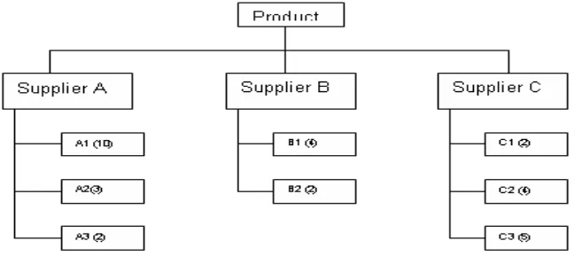
A case of three level supply chain involving n number of buyers, a single manufacturer and multiple suppliers is considered in this work. An individual buyer orders for finished products from manufacturer, where each finished product requires k number of parts that has to be supplied by the suppliers. The manufacturer has p suppliers to supply all k items. It has been assumed that the each supplier supplies a unique number of items ks
which is required for the assembly of finished product. The model presented here is, both for the case of no coordination and coordination where different players of the supply chain tries to optimize its cost locally and then jointly.
Figure 3.1 : A schematic diagram representing a three level supply chain with multiple suppliers, a single manufacturer, and multiple buyers.
Figure 3.2: Product tree structure 3.2 Assumptions and Notations
3.2.1 Assumptions
In this model formulation, we assume:
Demand is deterministic and constant over time, The product requires k items,
Shortages are not allowed,
Lead-time is zero at each level of the supply chain, Time horizon is infinite,
Each facility in the system has self decision making authority. Supply chain produces a single product.
3.2.2 Notations
The input parameters and decision variables for the three levels i.e. buyers, manufacturer, and suppliers are denoted by the subscripts b, m and s respectively.
Buyers
n number of buyers, where j = 1,2,…..,n
Dj annual demand rate for the jth buyer(units/year)
Ab,j order cost per cycle(monetary units – MU)
hb,j holding cost per unit per year(MU/unit/year)
Tj cycle time(year)
Qj order quantity(unit)
Manufacturer
Am fixed order/setup cost per cycle for the vendor(MU)
hm holding cost per unit of a finished product per year(MU/unit/year)
Co fixed cost per unit of the product(MU/unit)
λm,j an integer multiplier to adjust order quantity of the manufacturer to that og buyer j
k number of items required by the manufacture of the product to assemble one unit of the finished product.
am,j the cost of placing a purchase order for the ith item, i=1,2,…,k
ui number of units required in one unit of the finished product.
hm,j holding cost per unit per year for item i(MU/unit/year)
cm procurement(manufacture) cost per unit for the manufacturer,
where
c
c
c
u
i(
MU
/
unit
)
k 1 i
i 0 v
Suppliers:
p number of suppliers, where s=1,2,…,m
S the supplier’s number from whom the manufacturer procure I items As order cost for supplier s irrespective of the types of items ordered (MU)
hs,I holding cost per unit of time of item I supplied by supplier s (MU/unit/year)
Cs,I procurement cost per unit of the item I supplied by supplier s (MU/unit)
λs,j an integer multiplier to adjust the order quantity of supplier s for ks items to the order quantity of the
manufacturer.
k number of different types of items supplied by m suppliers. Note that k=
m 1 s sk
and each suppliersupplies unique items. That is, ks is supplier specific and never identical amongst suppliers.
Since the unit costs of materials are constant, they have no effect on the optimal policy and therefore are excluded from the cost functions of the buyers, manufacturer, and the suppliers. However, they are used in the numerical examples to compute the holding costs at the ends of the vendor and the suppliers.
3.3 Supply Chain Cost Calculations
when there is no coordination, each buyer determines its optimal order quantity, which is treated by the manufacturer as an input parameter. The manufacturer places orders to its suppliers in proportion to the individual buyer’s lot sizes. The suppliers deal with the manufacturer separately.
3.3.1 Buyer’s Annual Collective Cost Function
Suppose Buyer J orders Qj units from the manufacturer every T cycle of time. Then the total annual cost for a
buyer is the sum of the annual order cost and the annual holding cost, where T = Q/D Buyer’s total annual cost = annual order cost (A/T) + annual holding cost(hDT/2) Then the collective annual buyer’s cost function for n number of buyers is given by
n j j j j b jb
D
T
h
T
A
C
1 , ,2
(1)Where Tj* =
j
b
h
j
D
j
b
A
,
/
,
2
is the optimal cycle time for buyer j indicated by an asterisk (*).3.3.2 Manufacturer’s Annual Cost Function
When there is no coordination, it is assumed that the manufacturer manages each buyer separately. It delivers the finished product as per the economic lot size of the individual buyers. The manufacturer’s annual cost to satisfy the order of buyer j is
parts
and
items
finished
the
of
cost
holding
Annual
parts)
(including
cost
ordering
Annual
cost
annual
s
er'
Manufactur
j j k 1 i i i , m j j m j k 1 i i , m mm
D
T
2
u
h
T
D
2
h
T
a
A
C
(2)The manufacturers total cost is the sum for n buyers, and is given as
n 1 j j j k 1 i i i , m n 1 j j j m n 1 j j k 1 i i , m m n 1 j mm
D
T
2
u
h
T
D
2
h
T
a
A
C
C
(3)Where the terms
j k 1 i i , m m
T
a
A
= the manufacturer’s annual order cost
j j m
T
D
2
h
= the holding cost to meet annual demand for buyer j
j j k 1 i i i , m
T
D
2
u
h
= holding cost of items required for assembly to meet buyer’s jth demand
3.3.3. Suppliers Annual Cost Function
The manufacturer has p suppliers to supply all k items. When a buyer places an order of size Qj with the
manufacturer then the manufacturer will decide its order quantity for a particular supplier. This way p supplier has to provide all k items.
n 1 j j j k 1 i i i , s j ss
h
u
D
T
Where the terms As/Tj, and j j k 1 i i i ,
s
u
D
T
h
2
1
s
are respectively the annual order cost and holding cost for
supplier s to meet the annual demand for items requested by the buyers. The collective annual cost for p suppliers (
C
) is given by summing (4) for p number of suppliers
p 1 s n 1 j j j k 1 i i i , s j s p 1 ss
h
u
D
T
2
1
T
A
C
C
s (5)3.3.4 The Supply chain’s Annual Cost Function
The annual cost for uncoordinated supply chain is determined by summing the individual total cost for the buyers, manufacturer and the suppliers. Final Eq. (6) can be obtained by summing Eq.(1), (3) and (5).
(6)
3.4 Coordinated Supply Chain
When there is coordination the manufacturer consolidates the buyers order to minimize its cost. An optimal replenishment cycle time is calculated. For the coordination of the given three tier supply chain we need to introduce two integer multipliers λm,j and λs,j in order to adjust the demand quantities upstream.
3.4.1 Buyer’s Annual Collective Cost Function
The cost function of the buyers will be same as given by Eq. (1). The demand of the buyers will remain same as they are taken as the base in the backward coordination of the supply chain. Now the variable for the buyers will be the time function; which will now be dictated by the manufacturer. The orders of the individual buyers will be consolidated by the central player effecting coordination i.e. manufacturer. The cost function for n buyers is given as
n 1 j j j j , b j j , b b2
T
D
h
T
A
C
(1)3.4.2 Manufacturer’s Annual Cost Function
To effect coordination in the supply chain it is assumed that the manufacturer is the central player which coordinates the upstream and downstream inventories through a central plan. When buyer j places an order of size Qj with the manufacturer every Tj cycle of time, now to proceed towards coordination, the manufacturer
determines its order quantity λm,j Qj for a particular supplier i.e. the manufacturer will deliver orders in multiples
of the optimal lot size to a particular buyer.
The integral factor λm,j appears in denominator for the ordering cost and gets multiplied in the numerator for the
carrying cost. This is so because with increase in the lot size for the same demand the number of orders decreases and inventory increases. The total cost of the manufacturer hence will be given by Eq. (7)
m,j
j jk 1 i i i , m j j , m m j k 1 i i , m m j , m
m
1
D
T
2
u
h
T
D
1
2
h
T
a
A
C
(7)It can be easily seen that as λm,j increases, the total ordering cost decreases and total holding cost
increases(although in different proportion).
Then the manufacturer’s total cost is the sum for n buyers, and is given as
n 1 j j j j , m k 1 i i i , m n 1 j j j , m m n 1 j n 1j m,j j k 1 i i , m m j , m m m
T
D
1
2
u
h
T
D
1
2
h
T
a
A
C
C
(8)Where the terms
n 1j m,j j k 1 i i , m m
T
a
A
is the manufacturer’s annual order cost
n 1 j j j j , m mT
D
1
2
h
is the holding cost to meet annual demand for buyer j
n 1 j j j j , m k 1 i i i , m T D 1 2 u h is the holding cost of items required for assembly to meet jth buyers demand
3.4.3 Supplier’s Annual Cost Function
The manufacturer has p suppliers to supply all k items. Now similar to the previous procedure when buyer j places an order of size Qj with the manufacturer every Tj cycle of time, the manufacturer determines its order
quantity λm,j Qj for a particular supplier and places orders for k items to be supplied from p suppliers. For the
manufacturer to fulfill the order for buyer j, he will request ujλm,j Qj units of item i. Then the annual cost for
supplier s is written as
n 1 j j j j , s k 1 i i , s j , m j j , m j , s s j , ss
h
u
1
D
T
2
T
A
C
s
(9)Where the terms
j j , m j , s s
T
A
and
s,j
j jk 1 i i , s j , m
T
D
1
u
h
2
s
are respectively the annual order cost and holding cost for
supplier s to meet the annual demand for items requested by the manufacturer.
The collective annual cost for total suppliers is given by summing Eq. (9) for p number of suppliers
p 1 s n 1 j j j j , s k 1 i i i , s j , m j j , m j , s s p 1 ss
h
u
1
D
T
2
T
A
C
C
s
(10)3.4.4 Supply Chain’s Annual Cost Function
The annual supply chain cost is determined by summing the total cost of individual player. Equation (11) gives the total supply chain cost obtained by summing Eq.(1),(8) and (10).
p 1 s n 1 j j j j , s k 1 i i i , s j , m j j , m j , s s n 1 j j j j , m k 1 i i i , m n 1 j j j , m m n 1j m,j j k 1 i i , m m n 1 j j j j , b j j , b m b chain T D 1 u h 2 T A T D 1 2 u h T D 1 2 h T a A 2 T D h T A C C C C s
(11)If we consider a case where λs = λm = 1, i.e. considering a lot-for lot policy the holding costs for the suppliers
order according to given schedule, i.e. T=Qj/Dj, where j=1,2,….n Such a policy facilitates the consolidation of
the buyers order by the manufacturer.
For a coordinated supply chain in a centralized decision making we are assuming equal order cycle time for each buyer. As it has been observed from various literatures and earlier works that, in a decentralized decision making process which involves multiple decision makers, and where each decision maker tends to optimize its own performance, leads to an inefficient system. Therefore, like many works in the literature, this work also adopts the assumption of a centralized decision process, where there is a unique decision maker that manages the whole supply chain.
In the assumed scenario total annual cost of the supply chain can be rewritten as:
s k 1 j i s j p 1 s n 1 j s m p 1 s s s m j n 1 j k 1 j i i , m m n 1 j j m m m k 1 i j . m m n 1 j j j , b j , b chainu
h
D
1
T
2
A
T
1
D
2
u
h
T
1
D
T
1
2
h
T
a
A
2
T
D
h
T
A
C
(12)For this case of coordination the common optimum time T* for the buyers at which the total cost of the supply chain is minimum, can be evaluated by differentiating (12) with time T. This is justified as Eq.(12) is convex and differentiable over T, for every T ≥ 0.
Differentiating (12) with T and setting the first derivative to zero and solving for T, we have T*(λs, λv\ s =
1,2,….,m ) =
n 1 j p 1 s n 1 j k 1 i i i , s j s m n 1 j n 1 j k 1 i j i i , m j m m j j , b n 1 j k 1 i s p 1 s s s i , m m v j , b su
h
D
1
D
u
h
D
h
1
D
h
/
A
a
A
/
2
A
2
(13)4. METHODOLOGY AND NUMERICAL ANALYSIS
4.1 Methodology
The methodology of developing a model is a systematic path in which different tasks are performed and the output of one task is required for the input of the next task to be performed. The detailed methodology for the present work is as shown below.
Step 1: Detailed study of the supply chain and of various players of the supply chain. Step 2 : Capture the importance of coordination of various components of supply chain.
Step 3 : Exhaustive literature survey for coordination involving coordination among different players of the supply chain and the corresponding mathematical model.
Step 4 : Define the actual problem ailing the normal SC networks.
Step 5 : Propose a model to solve the problem underlining the research scope. Step 6 : Describe the assumptions and develop the mathematical model. Step 7 : Simulation of the model for the optimum results using software. Step 8 : Analysis of the results and discussions on the improvements.
4.2 Solution Procedures:
The following algorithm has been operationalized in this research. 1. Input the demands and cost of the buyers
2. Determine the optimal cycle time (T*) and economic lot size (Qj) for each buyer.
3. Buyer j orders Qj units from the manufacturer every Tj cycle time. Find the cost of one buyer and sum
it for n buyers.
4. The manufacturer determines its order quantity in the multiples of the economic lot of each buyer and places order quantity λm,j Qj for a particular supplier. This cost incurred has to be summed for n buyers.
As one finished product require K items to be supplied by p suppliers, where each supplier supplies Ks
items of unit ui. For the supplier to fulfil this required order from manufacturer, he will deliver uiλm,j Qj
4.2.1 For coordination
1. In normal supply chain T1≠ T2≠ …. ≠ Tn. To coordinate the supply chain the manufacturer must entice
the buyers to order according to a common schedule.
2. Initially we assume λs=p = … = λs=2 = λs=1 = λm = 1 and compute T* from eq.13. This common cycle
time is used in centralized decision making to manage SC..
3. Now we try to minimize the cost of the supply chain by optimkising the value of λs and λm.
4. Form eq.12 find Cchain(λs=p, …., λs=2, λs=1, λm ) = Cchain(1,…,1,1,1) = VALUE 1.
5. Let λm,2 = λm,1 + 1 = 2, compute T*.
6. Now set Cchain(λs=p,…,λs=2,λs=1,λm,2 ) = Cchain(1,…,1,1,2) = VALUE 2.
7. If VALUE 1 < VALUE 2, then values in step 4 are optimal values and corresponding T* is optimal time otherwise set Cchain(1,…,1,1,2) = VALUE 1.
8. Let λm,3 = λm,2 + 1 = 3, compute T*.
9. Now set Cchain(λs=p,…,λs=2,λs=1,λm,3 ) = Cchain(1,…,1,1,3) = VALUE 2.
10. Continue till Cchain(1,…,1,1, λm) < Cchain(1,…,1,1, λm+1) and Cchain(1,…,1,1, λm) < Cchain(1,…,1,1, λm-1).
11. Record this value as λs=p,…,λs=1 = 1, ,λs=2 = 1,λm* = b and , Cchain(1,…,1,1, b) = RECORD 1.
12. Now initiate λs=p, = 1,….λs=2 = 1, ,λs=1 = 2,λm = 1 with Cchain(1,…,1,2, λm*) = VALUE 1.
13. Repeat steps (5), (6), (7) till Cchain(1,…,1, λ*s=1 = 2, λm* ) < Cchain(1,…,1, λ*s=1 = 2, λm*+1 ) and
Cchain(1,…,1, λ*s=1 = 2, λm* ) < Cchain(1,…,1, λ*s=1 = 2, λm* - 1) and record the value as RECORD 2.
14. Repeat the same for other suppliers.
15. The minimum Cchain value is taken as optimum value.
4.3 Simulation
Nowadays computers are able to perform many different tasks, from simple mathematical operations to sophisticated animated simulations. But computer does not create these tasks by itself; these are performed following a series of predefined instructions that conform what we call a program. Simulation programme for finding the optimal solution is written with the features that, all code is based on standard C++ only. It does not need any non standard package, and can be compiled on all platforms.
4.4 Numerical Study
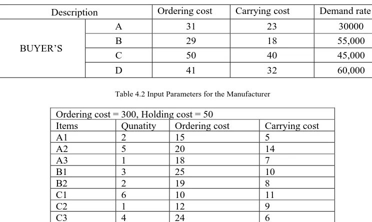
The numerical analysis for a three level supply chain consisting of four buyers, manufacturer and three suppliers is presented. The values for buyer’s ordering cost, holding cost and demand is varied from 20 – 50, 10 – 40 and 15000-60000 respectively. The values for manufacturer ordering and holding costs are varied from 50-100 and 20-50 respectively. The values for suppliers ordering cost and holding cost are varied from 10-30 and 5-15 respectively. The table 4.1 shows the respective cost parameters of the four buyers in the supply chain.
Table 4.1 Input Parameters for the Buyers
Description Ordering cost Carrying cost Demand rate
BUYER’S
A 31 23 30000 B 29 18 55,000 C 50 40 45,000 D 41 32 60,000
Table 4.2 Input Parameters for the Manufacturer
Ordering cost = 300, Holding cost = 50
Items Qunatity Ordering cost Carrying cost
A1 2 15 5
A2 5 20 14
A3 1 18 7
B1 3 25 10
B2 2 19 8
C1 6 10 11
C2 1 12 9
C3 4 24 6
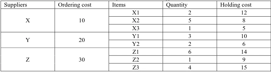
Table 4.3 Input Parameters for the Suppliers
Suppliers Ordering cost Items Quantity Holding cost
X 10
X1 2 12 X2 5 8 X3 1 5
Y 20 Y1 3 10
Y2 2 6
Z 30
Z1 6 14 Z2 1 9 Z3 4 15
4.5 Solution
For uncoordinated supply chain the total supply chain cost is 178168.92, the solution obtained for coordinated supply chain is obtained using the simulation run for the programme code.
Table 4.4 Results obtained for Different Integral Values in Coordination
S.No. λs1 λs2 λs3 λm T* Cchain
1 1 1 1 1 0.0142205 129697
2 1 1 1 2 0.00547931 150576
3 1 1 1 3 0.00459337 175159
4 1 1 2 1 0.00741702 132534
5 1 1 2 2 0.0054532 150443
7 1 2 1 1 0.00724722 121521
8 1 2 1 2 0.00721302 121385
9 1 2 1 3 0.00540062 150184
10 2 1 1 1 0.0073210 132861
11 2 1 1 2 0.0056321 168921
12 1 2 2 1 0.0056738 161290
13 1 2 2 2 0.0045274 174756
14 1 2 2 3 0.00397503 196329
15 2 1 2 1 0.006325 142140
16 2 1 2 2 0.00551392 150756
17 2 1 2 3 0.00381619 254071
18 2 2 1 1 0.00561448 162381
19 2 2 1 2 0.00455636 174627
20 2 2 1 3 0.00398171 196195
21 2 2 2 1 0.0045495 174888
22 2 2 2 2 0.00356785 215638
5. RESULTS AND DISCUSSIONS
In the previous chapter, a numerical study has been made explaining the algorithm. In the present chapter, the impact of varying lot sizes in coordination has been discussed where supply chain cost has been taken as a performance measure. A comprehensive analysis of the result is presented by using the cost data for supply chain and explaining the effect thereof. Various inferences drawn out of the results are mentioned at the suitable places. In the present study, the inventory cost, ordering cost, are taken as the different component of the total supply chain cost. Number of buyers and suppliers with a single manufacturer are the other parameters of variation in the supply chain.Various literatures in this framework have generally used excel spread sheets with VBA codes for the solutions. The solution presented here is obtained by coding in Borland C++ 5.02 enhanced with simulation tool pack.
5.1 Decentralized Case
When there is no coordination, each buyer determines its own optimal order quantity, which is treated by the manufacturer as its input parameter. The manufacturer places orders to its suppliers in multiples of the buyers order lot sizes. The suppliers deal with the manufacturer’s order separately. The values for costs are obtained by solving equations (1) – (6) in case of decentralized supply chain for the parameters as mentioned.
The values for buyer’s ordering cost, holding cost and demand is varied from 20 – 50, 10 – 40 and 15000-60000 respectively. The values for manufacturer ordering and holding costs are varied from 50-100 and 20-50
respectively. The values for suppliers ordering cost and holding cost are varied from 10-30 and 5-15 respectively. The results obtained from programme run is presented in table 5.1.
Table 5.1 Various Costs for the Decentralised Supply Chain
S.No Description Buyers Cost Manufacturer Suppliers Cost Total Cost
Case 1 2 buyers and 2 li
20334.3 55958.9 4796.75 81089.95 Case 2 2 buyers and 3
li
32102.9 72578.7 10912.6 115594.2 Case 3 4 buyers and 3
li
43135.2 174257 37548 254940.2 Case 4 5 buyers and 4
li
45504.8 272690 54092.5 372287.3 Case 5 6 buyers and 4
li
65778.1 275253 58999.45 400030.6
Case 6 7 buyers and 5 li
69878.8 280291 67012.32 417182.1
The figure 5.1 shows the average percentage share of the total cost among the various players of the supply chain for uncoordinated case. The result shows that for the given system, the manufacturer has the highest share of 62% in case of no coordination. The average cost percentage is minimum for the buyers with 17% followed by suppliers 21% of the total supply chain cost.
Average Percentage Share of Total Supply Chain Cost
62% 17%
21%
Manufacturer Cost Buyer's Cost Supplier's Cost
Figure 5.1: Percentage Share of total supply chain cost for decentralized case 5.2 Centralized Case
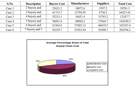
Table 5.2 Various costs for the coordinated Supply chain
S.No Description Buyers Cost Manufacturer Suppliers Total Cost
Case 1 2 buyers and li
25621.2 10072.6 3597.5 39291.3 Case 2 2 buyers and
li
41733.7 13789.95 8730.2 64253.85 Case 3 4 buyers and
li
55213.1 34851.4 33793.2 12387.7 Case 4 5 buyers and
li
56881.6 49084.2 37864.7 143830.5
Case 5 6 buyers and li
81564.8 57803.13 46019.5 185387.4 Case 6 7 buyers and 5
li
92239.7 51853.84 58300.7 202394.2
Average Percentage Share of Total Supply Chain Cost
22%
46% 32%
Manufacturer Cost
Buyer's Cost
Supplier's Cost
Figure 5.2 Percentage Share of total supply chain cost for centralized case
In case of coordination among the players, the share of their cost is shown in figure. It is interesting to note that the structure of the cost percentage has been changed significantly. The downstream buyers now have maximum share of 46% and manufacturer share have reduced to minimum of 22%. The suppliers cost share has changed to 32%. This shows the effect of coordination in this case result in cost reduction of manufacturer by impressive 64.5%. It is important to note that the cost of the supply chain, which is less than the total supply chain cost for decentralized case.
5.3 Centralized Vs Decentralised
To be able to see, how much of the coordination potential our approach can capture for a given problem, we first look at the difference between total costs of the system for pre-coordination replenishment policy obtained using the decentralized lot sizing model and total cost in the centralized case. The figure shows the average cost comparison of the supply chain system in two cases of coordination and no coordination. The data is taken as average of the ten results obtained for same supply chain with variation in demand, ordering cost and holding cost keeping the quantity of items same. The result is obtained using simulation programme.
Average Cost Comparision of Supply chain
0 100000 200000 300000 400000 500000 600000 700000 800000
3 buyers 4 buyers 5 buyers 6 buyers 7 buyers
To
ta
l C
os
t
Coordination No Coordination
Fig.5.3average cost comparison of the supply chain system in two cases of coordination and no coordination
demand and cost parameters. We can say that the coordination becomes more important for big and complex supply chains and the cost reduction obtained is more projected for the same.
The three level supply chain considered can be varied in the ordering cost, holding cost and the number of parts required for manufacturing single product for variable number of buyers and suppliers with a single manufacturer. The values for buyer’s ordering cost, holding cost and demand is varied from 20-100, 10-40 and 15000-100000 respectively. The values for manufacturer ordering and holding costs are varied from 50-100 and 20-50 respectively. The values for suppliers ordering cost and holding cost are varied from 10-30 and 5-15 respectively. The results obtained for the supply chain system for 3 suppliers each supplying two different items is summarized in table below.
Table 5.3:Total cost comparision of centralized and decentralized systems
Description Model Total Buyers Total f
Total S li
Total system With 2 buyers Decentralised 7322.89 33361.33 2918.59 43602.78
Centralised 9592.98 7673.09 2043.01 19309.08
With 3 buyers Decentralised 14242.1 61857.18 7572.38 83671.58
Centralised 18372.31 13917.86 5224.94 37515.11 With 4 buyers Decentralised 28671.5 120657 33469.3 182708.03
Centralised 37846.38 25198.50 23093.97 86138.85 With 5 buyers Decentralised 48773.5 284151 31448.9 364373.4
Centralised 64868.75 56261.89 22328.72 143459.36 With 6 buyers Decentralised 55670.8 254878.10 30616.2 341165.1
Centralised 73484.4 49701.22 20819.02 144004.64 With 7 buyers Decentralised 60579.6 390782 57940.1 509301.7
Centralised 81176.6 73467.01 41137.47 195781.08 With 8 buyers Decentralised 89670.7 407158 78245.2 575073.9
Centralised 121055.4 73288.44 53989.18 248333.02
The results show that the coordination leads to reduction in the total cost of the system in all the cases. This presents a clear need to adapt coordination mechanism, through consolidation of orders from buyers.
Table: 5.4 Total cost comparison in different cases
Description Buyers saving Manufacturer i
Suppliers saving Total system’s i
Case 1 -2270.09 25688.24 875.58 24293.7
Case 2 -4130.21 47939.32 2347.44 46156.47
Case 3 -9174.88 95368.50 10375.56 96569.18
Case 4 -16095.25 227889.11 9120.18 220914.04
Case 5 -17813.6 205176.88 9797.18 197160.46
Case 6 -20597 317314.99 16802.69 313520.62
Case 7 -31384.7 333869.56 24256.02 326740.88
Average Saving -14495.1 179035.2 10510.66 175050.8
6.Conclusion
in the centralized case. The suggested model achieves coordination amongst the members in a supply chain assuming common cycle time for all non identical buyers. This facilitates the consolidation of orders by the vendor and subsequently by the suppliers. Consolidation of orders in a supply chain results in reducing the order processing costs of the chain members; while fulfilling the annual demand. The numerical results indicated that the centralized case leads to savings fro the manufacturer, suppliers and the whole system as compared to the decentralized case. The results obtained for various cases showed on an average an impressive 54% saving for the manufacturer. However, centralized decisions induce losses for the buyers. These losses are the reason for which we proposed a mechanism for the warehouse to share its saving through discount quantity in order to cover retailer losses.
References:
[1] M.Ozbayrak, T.C. Papadopoulou, M. Akgun, “ Systems dynamics modeling of a manufacturing supply chain system” , Simulation modeling practice and Theory 15 (2007) 1338 – 1355.
[2] M.Y.Jaber, and S.K.Goyal, “ A basic model for co-ordinating a four level supply chain of a product with a manufacturer, multiple buyers and tier-1 and tier-2 suppliers”, International Journal of Production Research, (2008) 1-14
[3] M.Y. Jaber, and I.H. Osman, “ Co-ordinating a two level supply chain with delay in payments and profit sharing” Computers & Industrial Engineering, 50(2006) 385-400.
[4] Muckstadt, J.A., and Thomas, L.J., “Are multi-echelon inventory methods worth implementing in systems with low demand rate items?”, Management Science 26/5 (2002) 483-494.
[5] N erkip, W.H.Hausman, and S Nahmias; “Optimal centralized ordering policies in multi echelon inventory systems with correlated demands”, Management Sceince 36/3 (1998) 381-392.
[6] P.Coyle, P.A. Millerb, A.Y.Akbulut, “Coordinating ordering/shipment policy for buyer and supplier: Numerical and empirical analysis of influencing factors” International Journal pf Production Economics 108 (2002) 100-110.
[7] S.Sinha and S.P.Sarmah, “Supply chain coordination model with insufficient production capacity and option for outsourcing” Mathematical and Computer modelling 46 (2007) 1442-1452.
[8] S.Viswanathan; Rajesh piplani; “Coordinating supply chain inventories through common replenishment epochs” European Journal of Operations Research 129 (2001) 277-286.
[9] S.W.Kim and S.Park, “ Development of a three echelon SC model to optimize coordination costs” , European Journal Operation Research 184 (2008) 1044-1061.
[10] S.P.Sarmah, D.Acharya, S.K.Goyal, “Buyer vendor coordination models in supply chain management” European Journal of Operation Research 175 (2006) 1-15.
[11] Svoronos, A., and Zipkin, P., “Evaluation of one for one replenishment policies for multi echelon inventory systems”, Management Science 37/1 (1999) 68-83.
[12] Thomas, M.S. Neiro and Jose Griffin; “A general modelling framework for the operational planning of petroleum supply chains”, Computers and Chemical Engineering 28 (1996) 871-896.