A SOM based Incremental Clustering Algorithm

A SOM based Incremental Clustering Algorithm

Lei Chen

International Business Faculty, Beijing Normal University, Zhu Hai, China School of Management, Harbin Institute of Technology, Harbin, China

Email: [email protected]

Bao-Jin Zhao

School of Sports Leisure, Beijing Normal University, Zhu Hai, China Email:[email protected]

Li-Na Zhao

International Business Faculty, Beijing Normal University, Zhu Hai, China Email: [email protected]

Abstract—Due to fast development of network technique, internet users have to face to massive textual data every day. Because of unsupervised merit of clustering, clustering is a good solution for users to analyze and organize texts into categories. However, most of recent clustering algorithms conduct in static situation. That indicates, it doesn’t allow clustering algorithm to deal with novel data efficiently. When novel data appear, traditional clustering algorithms can’t change their structure easily. Obviously, this restrict is not fit to internet, since novel data appear at any time. For this reason, an incremental clustering algorithm is proposed in this paper to cluster incremental data. This algorithm has two factors. (a) It designs two measures to calculate feature’s ability and integrate them in similarity ment by replacing concurrence based similarity measure-ments. (b) Based on proposed similarity measurement, this algorithm selects few samples from original texts to perform incremental clustering. Experimental results demonstrate that, after integrating feature’s capacity, our algorithm can obtain high quality to cluster texts.

Index Terms—Self-organizing-mapping, feature’s intra-cluster representative ability, feature’s inter-intra-cluster discri-minable ability, similarity calculation

I. INTRODUCTION

Along with fast evolvement of internet technology, users have to face to massive texts from internet every day. This situation forces the issue that digs useful information from Word-Wide-Web has gradually became a headache problem. Recently, there are two possible ways for analyzing texts from web, and proposed many methods based these two ways. One is classification. The other is clustering. Comparing to clustering, classification is more accurate, whereas, classification needs to be provided with sufficient training data, and also needs some predefined labels. Obviously, this requirement is uneasy to be met in internet. For this reason, it enables

clustering prevalent for analyze web texts. Clustering needs no predefined knowledge. It runs all by data’s distribution to partition data into several classes. Among the classes, similar data are included by the same class, and dissimilar data are included by well-separated classes. Due to unsupervised merit of clustering, it is a good solution for users to analyze web information. Besides, clustering can be applied in many other fields, such as information retrieval, and web mining [1~2].

In fact, most of traditional clustering algorithms focus on static environment. It doesn’t allow adding any incremental data when clustering algorithm begins. Obviously, this restriction is too strict. Thus, some clustering algorithms for efficiently dealing with novel data are proposed [3]. They can be partitioned into two categories. One of them integrates incremental data and original data together to perform clustering. This plan is fit to any existent clustering algorithm, which just lets clustering algorithm run once more for data set including novel data and original data. Obviously, this plan is time-consuming [4, 5]. The other category forms a model from original data at first. When novel data appear it adjusts this model to make it not only fit to original data but also fit to novel data [6]. The methods in [7] and [8] are just based on this plan. However, they suffered from some drawbacks. One is that, they didn’t import feature’s capacity in clustering algorithms, thus, can’t obtain high-quality performance. The other is that, both of them neglected optimization analysis, which can’t confirm convergence of clustering algorithm.

To our knowledge, the most important factor to obtain good quality is to design an effective similarity measure ment. Recently, vector space model is the most popular text representative model [9]. As a result, it forces vector based similarity measurements, e.g. Euclidean distance, Cosine, KL, etc, generated from this model, become prevalent. Unfortunately, this kind of measurements regards any feature as identical. This phenomenon causes many noisy and useless features to affect similarity results and deeply depress clustering performance.

Corresponding author: Bao-Jin Zhao

To deal with aforementioned problems with traditional clustering algorithms, this paper proposes a feature’s capacity based clustering algorithm. This algorithm first uses self-organizing-mapping algorithm (SOM) to cluster original data, where each neuron corresponds one cluster. For dealing with novel data, this paper designs two abilities to measure feature’s capacity. They are: (a) feature’s intra-cluster representative ability to measure feature’s ability to aggregate similar data; (b) feature’s inter-cluster discriminating ability to measure feature’s ability to discriminate data into different clusters. Experi-mental results demonstrate that this kind of measurements can reflect similarities among texts more exactly. Furthermore, based on it, only few samples are needed to performance incremental clustering.

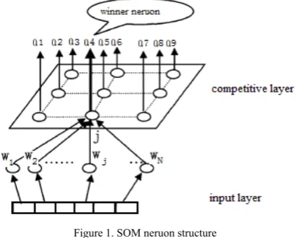
This paper uses self-organizing-mapping (abbreviated as SOM) to construct initial model from original data. SOM is first proposed by Kohonen [10]. It is an unsupe-rvised self-learning network and can reach high quality by iteratively tuning process. Neuron vector is used to represent cluster in this algorithm; one entry in this vector corresponds to one feature in vector space. Neuron struct-ure of SOM is shown in Fig.1.

Figure 1. SOM neruon structure

As Fig.1 shows, SOM often has two layers. The first layer is competitive layer and the second layer is input layer. Each input datum in the second layer has relations to each neuron in the competitive layer. To abbreviate relations in this figure, only the relations between the dimensionality-wj of input datum and each neuron in competitive layer are shown.

II.CLUSTERING BASED ON SOM

To cluster original data, we use the following equation. This equation is extensively used in SOM as optimization objective. When the difference between two values of Eq.1 respectively acquired from two successive steps falls below a predefined threshold, clustering algorithm stops. In this paper, we also use it as our optimization objective.

1

2 2

;

1 1

( ) ( )

( ) ( )

j i

j i

j i

v

d c

l

v v

d D c C

d c

l l

V l V l op

V l V l

=

∈ ∈

= =

=

∑

∑

∑

∑

(1)

Where, D denotes text collection for clustering and dj denotes one text in D; C denotes cluster set and ci denotes one cluster in C; Vdjand Vci respectively denote text vector and cluster vector formed from dj and ci; v denotes vector dimension; Vdj(l) and Vni(l) respectively denote the weights of lth entry in Vdjand in Vci.

To cluster texts by reducing the value of Eq.1, we use the iteratively tuning process similar to self-organizing-mapping (SOM) algorithm. To apply iteratively tuning process borrowed from self-organizing-mapping, the only thing needed to be done is to treat one cluster as one neuron, and treat cluster vector as neuron vector. Tradi-tional self-organizing- mapping based algorithms need to predefine an initial parameter, namely neuron topology. This topology should be identical with the distribution of the texts prepared for clustering. Obviously, it is uneasy to be accurately predefined unless we own the inherent knowledge about input data.

Thereby, some scalable self-organizing-mappingbased algorithms are proposed, such as GSOM [11] and GHSOM [12], which free of topology prediction. Between them, GHSOM consumes much time to cut clustering results generated by GSOM into several layers, whereas, this hierarchical structure brings in little improvement if we adopt it. Thus, the simple planar topology applied by GSOM is adopted by us.

GSOM just adopts Eq.1 as its optimizaton objective. After several iterative steps (often set as 100 according to [11]), when the difference between two values of Eq.1 respectively acquired from two successive steps falls below a predefined threshold (often set as 0.0001 also according to [11]), GSOM stops and regards one neuron as one cluster. On the opposite, when the difference of Eq.1 is beyond the threshold after 100 iterative steps, GSOM measures each neuron’s cohesion by Eq.2 and selects the neuron of the least cohesion and its neighbour, which has the least cohesion in the four neighbours. After selection, GSOM inserts new line of neurons between two columns respectively including these two neurons.

1

2 2

( )

1 1

( ) ( ) ( ) ( )

j i

j i i

j i

v

d n l

v v

d n c

d n

l l

V l V l op

V l V l

=

∈

= =

=

∑

∑

∑

∑

(2)

Where, ni denotes the neuron corresponding to the cluster ci; Vniis neuron vector formed from ni and is equivelent to Vci formed from ci; dj denotes one text included by cluster ci.

1..

( )

( )

( )

2

e d

r

n n

n l v

V l

V l

V l

=

+

=

(3)

Where, v denotes vector dimension; Vnr(l) denotes the weight of lth entry in nr, whichis the mean between Vne(l) and Vnd(l), the weights of lth entry respectively in Vne and in Vnd.

III.EVALUATION ON FEATURE’S CAPACITY

To our knowledge, SOM and its varieties often employ Cosine to compute similarity between input data and neuron, and regard each feature of identical importance in similarity measurement.

Let U denote text collection prepared for clustering. Let F denote vector space constructed from U. The clusters formed from U are labeled as {C1, C2,…, Ck}, where C1∪C2∪ ∪... Ck =U andCi∩Cj = ∅ . Let {F1, F2,…, Fk} denote set collection. Each feature set among {F1, F2, …, Fk} includes the features in F, which can represent the theme expressed by one cluster among {C1, C2,…, Ck}. For example, Fi only contains the features that are capable to represent the theme of Ci.

In fact, in text clustering:

a) The quantity of the features that are capable to represent the theme of one cluster is much smaller than the dimension of vector space. For example, if there is one cluster whose theme is about “sport”, to represent it, it only needs the features, whose meanings are relevant to “sport”, such as “score”, “ball” or “athlete”. Thus, each feature set among {F1, F2, …, Fk} is much smaller than F.

b) The larger is vector space, the more semantically similar features it includes. Therefore, when vector space is large enough, most of features in it are semantically related. If we sample one to represent all of them, each set among {F1, F2, …, Fk} is much smaller than F.

To wipe out the effects on similarity measurement brought from irrelevant and noisy features, two measures are proposed to assign them to weights in similarity measurements, which are illustrated by Eq.4 and Eq.6. These two equations respectively measure feature’s ability to represent the theme of one cluster and the ability to separate one cluster from the others.

Eq.4 measures feature’s intra-cluster representative ability to represent the theme of one cluster. In other words, this ability stands for feature’s capacity to aggregate similar texts into one cluster.

2 2

| | | | | |

1 1&& 1

( ) ( ) ( ) ( )

( , )

( ) ( ) ( ) ( )

i i i

p q p i

p q p i

c c c

d d d n

l i

p q p q d d p d n

V l V l V l V l

InTraCM f n

V l V l V l V l

= = ≠ =

⎛ − ⎞ ⎛ − ⎞

⎜ ⎟ ⎜ ⎟

= _{⎜ ⎟} + _{⎜ ⎟}

+ +

⎝ ⎠ ⎝ ⎠

∑ ∑

∑

(4)

Where, cidenotes the cluster which includes the texts that are more similar to the neuron ni than to the other neurons; |ci| denotes the volume of ci.. The other symbols are already explained in Eq.1.

Two intuitive ideas can help explain why previous equation is tenable to measure feature’s ability to represent the theme of one cluster:

a) If one feature (e.g. fl) is assigned to similar weights among the texts included by one cluster (e.g. ci), fl certainly can help aggregate similar texts into ci comp-actly. The part before the plus of Eq.4 forms according to this idea.

b) As traditional self-organizing-mapping based algori-thms, neuron in our algorithm also represents cluster center. Then, if the weight of fl in each text included by ci is similar to the weight of fl in ni, fl certainly can help assemble similar texts around the cluster center of ci. The part after the plus of Eq.4 forms according to this idea.

In fact, if one feature has larger intra-cluster represent-ative ability, it will be assigned to smaller value by Eq.4. Thus, Eq.4 is reversed to

max( ( , ));

( , )i ( , )i

l b b

l l

InTraCL InTraCM f n

InTraC f n InTraCL InTraCM f n

=

= − (5)

Eq.6 measures feature’s inter-cluster discriminable ability to distinguish one cluster from the others.

2

1&&

( , )l i k | n_i( ) n_b( ) |

b b i

InTerD f n V l V l

= ≠

=

∑

− (6)

Where, k denotes the quantity of the neurons.

Eq.6 forms based on the idea, that the weight of one feature in one neuron vector is the mean weight of that feature among the texts mapped to that neuron [13]. Our algorithm also obeys it. Then, if one feature has distinct weights among most of neuron vectors, this feature can help separate clusters far away from one another.

A parameter λ is set to combine aforementioned two measures together.

( , )_{l i} * ( , ) (1 )*_{l i} ( , )_{l i} CA f n =

λ

InTraC f n + −

λ

InTerD f n (7) Where, λshould be set by user’s choice. Nevertheless, since we don’t have sufficient transcendental knowledge, we intuitively set λ as 0.5, which also indicates that intra-cluster representative ability and inter-intra-cluster discrimi-nable ability are both important for selecting features.

After calculating feature’s ability by Eq.7, we can import feature’s ability in similarity measurement.

IV.INCREMENTAL CLUSTERING

As indicated in [14, 15], the best way to perform incremental clustering is to integrate incremental data and samples selected from original data together to adjust clustering model generated from original data. In order to perform this plan, the important task is to devise an effective sample selecting plan.

A. Sample Selection

den-sity clustering algorithms, there need to predefine two parameters and sensitive to these two parameters. They are the diameter of neighborhood E and the minimal points-MinPts in neighborhood E [16]. However, they are hard to be predicted. Thus, this paper employed its improved version-“local density” to partition data into several intra-clusters and select samples by partition results [17].

After each cluster is separated into some sub-clusters, M samples are selected to represent each sub-cluster by relation results from Eq.8.

In order to select samples, the Best Matching Neuron (BMN) and the Second Matching Neuron (SMN) are integrated in computation. Where, BMN stands for the neuron which has the max similarity to Dj. SMN stands for the neuron which has the second similarity to Dj.

( , ) - ( , )

( , )

( , ) ( , )

j j

j

j j

Sim D BMN Sim D SMN

Relation D BMN

Sim D BMN Sim D SMN

=

+ (8)

If the difference between Sim(Dj,BMN) and Sim(Dj,SMN) is larger, it means Dj is more similar to the cluster which Dj belongs to, and has less similarity to other clusters. It also demonstrates that Dj locates at the center area of the cluster which it belongs to. When novel data appear, Dj may not easily move to another cluster.

On the contrary, if the difference is smaller, it means Dj locates at the boundary area of the cluster which Dj belongs to. When novel data appear, Dj may easily move to another cluster.

Except for aforementioned two data, it also needs another datum, whose relation is between the max and the least, to represent the data locate at the middle area of the sub-cluster. Therefore, it can be concluded that, with previous precise similarity measurement, it only needs M equal to 3.

B. Incremental Clustering

When incremental data appear, the samples selected from original data can be combined with incremental data to adjust neuron model.

In text clustering, the features, which can represent the theme of the text or the cluster, are really effective in similarity calculation, whereas, the other irrelevant features not only prolong running time but also depress clustering performance. For this reason, we propose an intersection based similarity measurement to address this problem. This measurement is effective for dealing with incremental data. In this measurement, only the intersec-ted features, which are both assigned to non-zero weights in text vector and neuron vector, are considered by our similarity measurement as Eq.9 shows. Besides, the feature’s capacity is also integrated in this similarity measurement.

Actually, our algorithm applies tuning process similar to SOM. In this process, to accelerate clustering velocity and improve clustering performance, it assigns the features, whose abilities are larger than mean value, to non-zero weights. Then, if many features are of non-zero weights in both text vector and neuron vector, it indicates that the text and the neuron share the similar theme.

Eq.9 just forms based on this idea.

( ) 0&& ( ) 0

2 2

( ) 0 ( ) 0

( ) ( )

( , ) *log( , )

( ) ( )

j i

dj ni

j i

dj ni

d n

V l V l

j i l i

d n

V l V l

V l V l

Sim d n f n

V l V l

≠ ≠

≠ ≠

=

∑

∑

∑

(9)

Where, ni denotes ith neuron in neuron set; dj denotes jth text in text collection; fl denotes lth feature in vector space; Vni denotes neuron vector formed from ni; Vdj denotes text vector formed from dj; Vdj(l) denotes the weight of lthentryin Vdj, which is evaluated by TF-IDF; Vni(l) denotes the weight of lthentryin Vni.

To fine-tune feature’s weight in neuron vector, our algorithm applies iteratively tuning process to adjust the winner neuron and its adjacent neighbors. The detailed tuning process is specified by [13], where concurrence based similarity measurements, e.g. Euclidean distance, Cosine, KL, are applied as their standard similarity measurements. Since our algorithm uses Eq.9 as its similarity measurement, its neuron adjustment function needs also to be changed as:

( ) ( ) ( )

( )( ) ( ) * * ( ); ( ) ( ) ( ) 0 & & ( ) 0

( )( 1)

1.0;

( ) 0 & & ( ) 0

j i

i

j i

j i

i

j i

d n

n

d n

d n

n

d n

V l V l NH t

V l t a t

dist V l V l If V l V l

V l t

If V l V l

− ⎧

+

⎪ ₊

⎪

⎪ _{≠ ≠}

+ =⎨ ⎪ ⎪

⎪ _{≠ =}

⎩

(10)

Where, Vni(l)(t+1) and Vni(l)(t) respectively denote the weights of the feature fl in neuron vector Vni after and before neuron adjustment; a(t) denotes learning rate, and descends along with tuning process; dist and NH(t) denote distance function and neighborhood range.

Eq.10 is divided into two parts aiming at dealing with two situations. They are:

a) If one feature (e.g. fl) whose weights are both non-zero in two vectors respectively formed from text and neuron (e.g. dj and ni), the upper sub-equation is applied to adjust feature’s weight in ni.

b) Since many features are assigned to zero weights by our algorithm, it is easy to occur that some features’ weights are non-zero in text vector and zero in neuron vector. Then, the lower sub-equation is utilized to assign them to an initial weight.

V. EXPERIMENTS AND ANALYSES

TABLE 1. DATA SET DETAILS Data

set

Numerical feature

Continuous feature

Boolean feature

Data volume

Class number

Iris 4 -- -- 150 4

Glass -- 9 -- 214 7

Wine -- 13 -- 178 3

Zoo 2 -- 15 101 7

In order to compare the precisions of different clusteing algorithms, three metrics are employed. They are Purity, NMI (Normalized Mutual Information) and ARI (Adjusted Random Index) respectively introduced in [19~21]

Eq.11 is purity result corresponding to one cluster, e.g. Sr.

Eq.12 is its algebraic mean through all the clusters, which can estimate the precision of clustering algorithm.

1

1

( )

max( )

k q

r _q r

r

P S

n

n

=

=

(11)

1 1

max( )

k k

q r q

r r

k

Purity

n

n

=

=

=

∑

(12)

Eq.13 is NMI result, which is calculated based on entropy. Since NMI doesn’t need to predefine cluster number, and utilizes inter-cluster distinctness and intra-cluster agglomeration to measure intra-clustering results, it’s extensively applied in clustering evaluation scenario.

1 1

1 1

*log( * * )

*log( ) *log( )

2

k k

q q q

r r r

r q

k k

q q

r r

r q

n n n n n n

NMI

n n n n n n n n

= =

= =

=_{⎡ ⎤}

+

⎢ ⎥

⎣ ⎦

∑∑

∑

∑

(13)

Where, Sr denotes rth cluster acquired by clustering algorithm; nr denotes the quantity of the texts included by Sr; Cq denotes qth cluster predefined by user; nq denotes the quantity of the texts included by Cq;

n

_rq denotes the quantity of the texts included by the intersection between Cq and Sr; n denotes set size; k denotes cluster number.

Unfortunately, Purity and NMI need to relate the labels indicating the clusters acquired by clustering algorithm to the labels predefined by user, whereas, it is infeasible in operation for large-scale text collection. When text collection expands, cluster number also increases mean-while. In this situation, it’s difficult to define which cluster’s label formed by clustering algorithm corres-ponds to which class’s label predefined by user. There-fore, we import ARI (Adjusted Random Index) to deal with this situation, which evaluates how well the algori-thm splits input data into different clusters by looking at the relation between clusters and not between clusters and the given labels.

With respect to ARI, it combines two texts as one pair-point. If the volume of text collection is n, this collection has n*(n-1)/2 possible pair-points. It utilizes four situations to identify clustering results.

a) Two texts included by one pair-point are manually labeled in the same cluster, and in clustering results they are also in the same cluster.

b) Two texts included by one pair-point are manually labeled in the same cluster, and in clustering results they are in different clusters.

c) Two texts included by one pair-point are manually labeled in different clusters, and in clustering results they are also in different clusters.

d) Two texts included by one pair-point are manually labeled in different clusters, and in clustering results they are in the same cluster.

Let the numbers of the pair-points which meet previous four situations as a, b, c, and d. Apparently, a and c stand for the rightly partitioned pair-points, and can be used to measure clustering precision as

2

( ) [( )( ) ( )( )]

2

[( )( ) ( )( )]

2 n

a c a b a d b c c d

ARI n

a b a d b c c d

⎛ ⎞

+ − + + + + +

⎜ ⎟ ⎝ ⎠

=

⎛ ⎞

− + + + + +

⎜ ⎟ ⎝ ⎠

(14)

Eq.14 can better deal with the problem that the expected value of RI (Random Index, original version of ARI) of two random partitions does not take a constant value or that RI approaches its upper limit as the number of clusters increases.

Three clustering algorithms, such as K-means [22], GSOM [12], and BIRTH [23], are used as baselines. Clustering results of them are shown in Table 2. We use symbol SOMICA to stand for our clustering algorithm.

TABLE 2.

CLUSTERING RESULTS OF DIFFERENT ALGORITHMS

BIRTH K-means GSOM SOMICA

Iris

Purity 81.25 83.47 87.36 89.25

NMI 79.77 81.29 85.44 97.63

ARI 77.15 79.41 83.23 85.45

Glass

Purity 80.57 85.92 88.33 90.72

NMI 78.97 83.68 86.75 89.18

ARI 77.44 82.41 85.13 87.98

Wine

Purity 73.58 79.45 85.19 88.73

NMI 71.89 77.53 83.29 86.62

ARI 69.77 75.31 81.11 84.91

Zoo

Purity 76.53 83.37 87.44 92.38

NMI 74.39 81.30 85.31 90.25

ARI 72.01 78.94 83.14 87.79

these four algorithms. This is because, if texts are partitioned into certain cluster by BIRTH, they are never moved to any other cluster.

In order to measure the performance of our algorithm on clustering incremental texts, we use the large-scale text collection RCV1, including about 800K news stories already labeled by users and over one million features [24]. We partition this corpus into ten parts, and randomly select one part as original texts. The remaining parts are regarded as incremental texts. Thus, we can perform incremental clustering nine times, and one time, randomly select on part as incremental texts.

Since, the symbol SOMICA stands for the static version of our algorithm, we use SOMICA_IV to stand for its incremental version. In Table 3, SOMICA_IV is compared to SOMICA. Besides, the performances of GSOM, K-means and BIRTH are also listed.

TABLE 3.

CLUSTERING RESULTS OF DIFFERENT ALGORITHMS BIRTH K-means GSOM SOMICA SOMICA-IC

Purity 75.22 82.92 86.21 90.74 78.12

NMI 73.93 81.57 84.73 88.66 75.75

ARI 72.51 79.36 82.55 86.31 73.49

In this table, SOMICA and SOMICA_IV have similar results. That means, by integrating feature’s capacity in similarity measurement and removing irrelevant features, the incremental version of our algorithm still performs well comparing to the static version. Furthermore, its performance is close to GSOM, and far better than the other traditional static clustering algorithms, such as K-means, and BIRTH.

In Table 4, running time of different algorithms is compared.

TABLE 4.

RUNNING TIME OF DIFFERENT ALGORITHMS

Algorithm BIRTH K-means GSOM SOMICA SOMICA-IC

Time(s) 2228 693 746 783 921

In this table, running time of K-means is shortest. GSOM, SOMICA and SOMICA_IV follow closely. The reason is that, time complexities of K-means, GSOM, SOMICA and SOMICA_IV are all O (k′mn) [25]. k′ is cluster number, also is neuron number. m isrunning steps. n is data size. Since the rank of k′ from low to high is means, GSOM, and SOMICA. Thus, it has the rank as K-means, GSOM, and SOMICA. Since, SOMICA_IV is the incremental version of SOMICA, it runs SOMICA for several times. It certainly has longer running time than SOMICA, consequently, also longer than K-means and GSOM. BIRTH is one kind of hierarchical clustering, thus, it has the highest time complexity as O(n2_).

REFERENCES

[1] Xiao Q, Qian X D, Liao H. Clustering algorithm analysis of web users with dissimilarity and SOM neural networks. Journal of Software, 2012, 7(11): 2533-2537.

[2] Zhou X Y, Sun Z H, Zhang B L, Yang Y D. Research on clustering and evolution analysis of high dimensional data stream. Journal of Computer Research and Development,

2006, 43(12): 2005-2011.

[3] Sebastian L, Mihai L. Incremental clustering of dynamic data streams using connectivity based representative points. Data & Knowledge Engineering, 2009, 68(1): 1-27. [4] Asharaf S, Murty N M, Shevade S K. Rough set based incremental clustering of interval data. Pattern Recognition Letters, 2006, 27(6): 515-519.

[5] Li G S, Meng K, Xie J. An improved topic detection method for Chinese microblog based on incremental clustering. Journal of Software, 2013, 8(9): 2313-2320. [6] Zhang X H, Liu J Q, Du Y, Lv T J. A novel clustering

method on time series data. Expert Systems with Applications, 2011, 38(9): 11891-11900.

[7] Liu M, Liu Y C, Wang X L. IGSOM: Incremental

clustering based on self-organizing-mapping. The 8th International Conference on Intelligent Information Hiding and Multimedia Signal Processing, 2008: 885-890. [8] Cheng H J, Zhang G Y, Lou S J. A self-organizing maps

algorithm for gene expression data clustering based on feature's distribution. The 3rd International Conference on Advanced Computer Control, 2011: 307-310.

[9] Yang R L, Zhu Q S, Xia Y N. A novel weighted phrase-based similarity for web documents clustering. Journal of Software, 2011, 6(8): 1521-1528.

[10] T. kohonen.Self-organizing maps. Berlin: Springer, 1997, Chapter 3.

[11] Alahakoon D, Halganmuge S K, Srinivasan B. Dynamic self-organizing maps with controlled growth for knowledge discovery. IEEE Transactions on Neural Networks, 2000, 11(3): 601-614.

[12] Rauber A, Merkl D, Dittenbach M. The growing

hierarchical self-organizing map: exploratory analysis of high-dimensional data. IEEE Transactions on Neural Networks, 2002, 13(6): 1331-1341.

[13] Kohonen T, Kaski S, Lagus K, Salojarvi J, Honkela J, Paatero V, Saarela A. Self organization of a massive document collection. IEEE Transactions on Neural Networks, 2000, 11(3): 574-585.

[14] Pekpe K M, Lecœuche S. Online clustering of switching models based on a subspace framework. Nonlinear Analysis: Hybrid Systems, 2008, 2(3): 735-749.

[15] Srinivas, M, Mohan, C K. Efficient clustering approach using incremental and hierarchical clustering methods. The 2010 International Joint Conference on Neural Networks, 2010: 1-7.

[16] Ester M, Kriegel H P, Sander J, Xu X. A density-based algorithm for discovering clusters in large spatial data bases with noise. The 2nd International Conference on Knowledge Discovery and Data Mining, 1996: 226-231. [17] Ni W W, Sun Z H, Lu J P. K-LDCHD-A local density

based k-neighborhood clustering algorithm for high dimensional space. Journal of Computer Research and Development, 2005, 42(5): 784-791.

[18] Cathy Blake, Eamonn Keogh, Christopher Merz. UCI repository of machine learning databases. http://www.ics.uci.edu/~mlearn/MLRepository.html,

Irvine, CA, University of California, 1998.

[19] Zhao Y, Karypis G. Criterion functions for document clustering: Experiments and analysis, Technical Report, #01-40, 2002, University of Minnesota.

[20] Cilibrasi R, Paul Vitányi. Clustering by compression. IEEE Transactions on Information Theory, 2005, 51(4): 1523-1545.

[21] Hubert L, Arabie P. Comparing partitions. Journal of Classification, 1985, 2(1): 193-218.

Computational Statistics and Data Analysis, 2008, 52(10): 4658-4672.

[23] Qu J, Jiang Q S, Weng F F, Hong Z L. A hierarchical clustering based on overlap similarity measure. The 8th ACIS International Conference on Software Engineering, Artificial Intelligence, Networking, and Parallel/ Distributed Computing, 2007: 905-910.

[24] David D L, Yang Y M, Tony G R, Li F. RCV1: A new benchmark collection for text categorization research. Journal of Machine Learning Research,2004, 5: 361-397. [25] Shahpurkar S S, Sundareshan M K. Comparison of self-organizing map with k-means hierarchical clustering for bioinformatics applications. IEEE International Joint Conference Neural Networks, 2004: 1221-1226.

Lei Chen, China, Born in 1982. Ph.D Candidate.

Educational Background: Harbin Institute of Technology, Harbin, China.

Work Experience: International Business Faculty, Beijing Normal University, Zhu Hai, China.

Her main research interests include semantic similarity calculation and neuron processing.

Email: [email protected].

Previous Articles: Lei Chen, Baojin Zhao. A Novel Text Clustering Algorithm via Integrating Feature Set Construction and Text Partition. Journal of Computational Information System. 2013, 9(8).

Bao-Jin Zhao, Corresponding author, China, Born in 1980. Master.

Educational Background: Beijing Normal University, Beijing, China.

Work Experience: School of Sports Leisure, Beijing Normal University, Zhu Hai, China.

His main research interests include semantic similarity and web mining. Email: [email protected].

Li-Na Zhao, China, Born in 1962. Bachelor.

Educational Background: Changchun Institute of Technology University, Changchun, China.

Work Experience: International Business Faculty, Beijing Normal University, Zhu Hai, China.

Her main research interests include entity linking and neuron network.