Parameter Tuning via Kernel Matrix
Approximation for Support Vector Machine
Chenhao Yang, Lizhong Ding and Shizhong Liao
School of Computer Science and Technology / Tianjin University, Tianjin, China Email: [email protected]
Abstract—Parameter tuning is essential to generalization of support vector machine (SVM). Previous methods usually adopt a nested two-layer framework, where the inner layer solves a convex optimization problem, and the outer layer selects the hyper-parameters by minimizing either cross validation or other error bounds. In this paper, we propose a novel parameter tuning approach for SVM via kernel matrix approximation, based on the observation that approximate computation is sufficient for parameter tuning. We first develop a preliminary approximate computation theory of parameter tuning for SVM. We present a kernel matrix approximation algorithm MoCIC. We design an approximate parameter tuning algorithm APT, which applies MoCIC to compute a low-dimension and low-rank approximation of the kernel matrix, and uses this approximate matrix to efficiently solve the quadratic programming of SVM, then selects the optimal candidate parameter through the approximate cross validation error (ACVE). Finally, we verify and compare the feasibility and efficiency of APT on 10 artificial and benchmark datasets. Experimental results show that this new algorithm can dramatically reduce time consumption of parameter tuning and at the same time guarantee the effectiveness of the selected parameters. It comes to the conclusion that the approximate parameter tuning approach is sound, efficient, and promising.
Index Terms—kernel methods, parameter tuning, support vector machine, matrix approximation
I. INTRODUCTION
Support vector machine (SVM) is a theoretically well motivated algorithm developed from statistical learning theory. It is a significant learning system for efficiently training the linear machines in the kernel-induced feature spaces, while controlling the capacity to prevent overfitting by generalization theory [1].
Parameter tuning has an essential influence on the generalization performance of SVM. The traditional methods mainly adopt a nested two-layer framework [2] for choosing the optimal parameter, where the inner layer solves a convex optimization problem to obtain Lagrange multipliers for fixed values of the hyper-parameters including the kernel parameters and the penalty factor, and the outer layer adjusts the hyper-parameters by minimizing the estimates of generalization error, either cross validation [3]-[5] or other error bounds [6]-[8].
For 1-norm soft margin SVM, cross validation gives an
excellent estimate of the generalization error [3], but it demand a grid search over the parameter space, which unavoidably brings high computational complexity [9] because the inner convex optimization problem has to be iterated more times. So far, several approaches have been proposed to improve the efficiency of grid search, such as genetic algorithms [4] and evolution computation [5]. Approximate error bounds can also be taken as the criteria to select hyper-parameters. The commonly used bounds include span bound, Jaakkola-Haussler bound [7] and radius-margin bound [7], [8]. Generally, these two approaches take several strategies to reduce the search space of hyper-parameters to accelerate the outer layer of parameter tuning, then the inner-layer computation could be reduced of great quantity. Even so the determination of the search direction is usually of high cost and it is hard to verify the effectiveness of the search direction, and one iteration of the inner-layer’s computation stays unchanged. Furthermore, the complexity of quadratic programming for solving SVM is O n( 3) and that of second-order cone programming (SOCP) for multiple kernel SVM is O Nn( 3.5) [10], where n is the size of training examples and N is the number of candidate kernels. When it come to large-scale problems, it is prohibitive to directly train SVM for every candidate model, and it is desirable to design an algorithm that can improve the efficiency of parameter tuning based on the acceleration of the inner optimization.
approximate cross validation error (ACVE). Experiments on artificial and benchmark datasets suggest that APT can improve the efficiency of parameter tuning and at the same time guarantee the generalization performance of the selected parameters.
The rest of the paper is organized as follows. In Section 2, we give a brief introduction of SVM. In Section 3, we present the concept of kernel matrix approximation and also present the MoCIC. In Section 4, we propose the approximate parameter tuning algorithm APT and as well discuss its time complexity. In Section 5, experimental results show a comparison between parameter tuning algorithm with the original kernel matrix and with approximation of the kernel matrix gained by MoCIC. The last section gives the conclusion.
II. SUPPORT VECTOR MACHINE
We use to denote the input space and the output domain. Usually we will havep, { 1,1} for binary classification. The training set is denoted by
1, 1 , , ,
,n n n
y y
x x
where we refer to the xi as examples and the yi as their
labels, and n is the number of instances.
The maximal margin classifier is the basic model of SVM. It chooses the hyperplane ( , )wb that maximizes the classification margin for the linearly separable data. By solving the optimization problem
min , ,
s.t. , 1,
1, , ,
i i y b i n w w
w x (1)
we can obtain the hyperplane( , )w b .
The equivalent dual form of formula (1) is
, 1 1
1
1
min , ,
2
s.t. 0,
0, 1, , ,
n n
i j i j i j i
i j i
n i i i i y y y i n
x x (2)where i, j are the Lagrange multipliers.
Implicitly mapping the training data into the feature space defined by kernel K x z
, , we can obtain the kernel version of formula (2):, 1 1
1
1
min ( , ) ,
2
s.t. 0,
0, 1, , .
n n
i j i j i j i
i j i
n i i i i y y y i n
K x x
(3)
For the non-separable data in the feature space, we can obtain the optimum hyperplane by solving the following
optimization problem,
1 1
min , ,
2
s.t. ( , ) 1 , 0, 1, , .
n i i
i i i
i C y b i n
w ww x (4)
When using kernel trick the equivalent dual form of formula (4) is
, 1 1
1 1
min ( , ) ,
2
s.t. 0,
0, 1, , ,
n n
i j i j i j i
i j i
n i i i i y y y
C i n
K x x
(5)
where C is the penalty factor.
The formula (5) is equivalent to the following problem
T T T 1 min , 2 s.t. 0, 0, C Q e y (6)
where yn is the label vector, eis the n-vector of ones, the matrix[ ]Qij y yi jK x x( i, j) , and inequality
0
C means Ci 0,i1,,n. Denoting the solutions of problem by
*
, 1, , ,
i i n
the final hypothesis can be defined as
* 1
( ) sgn , .
n
i i i i
f y b
x K x x
From the above optimization formulae, we can find that the performance of SVM mainly depends on the Lagrange multipliers and the hyper-parameters. The Lagrange multipliers can be easily obtained through solving the quadratic programming when hyper-parameters are fixed, so the hyper-hyper-parameters have a decisive influence on the performance of SVM.
In this paper, we aim at developing an efficient method for the selection of hyper-parameters from the perspective of kernel matrix approximation.
III. KERNEL MATRIX APPROXIMATION
It is a fundamental result of linear algebra [14] that for any matrix A and positive integer k , there exists a matrix Ak. which simultaneously minimizes ‖AD‖ over rank k matrices D, for all norms that are invariant under rotation (for example, the Frobenius norm and the 2-norm). Ak is called the optimal rank k approximation,
The objective of kernel matrix approximation is to design an efficient algorithm to obtain a near-optimal low-rank approximation of the kernel matrix satisfying
,
k k
A A A A
‖ ‖ ‖ ‖
where represents a tolerable level of error for the given application.
A. Algorithm MoCIC
In this paper, synthesizing the Monte Carlo algorithm [11],[12] and incomplete Cholesky factorization [15], we develop a kernel matrix approximation algorithm MoCIC (Monte Carlo algorithm and incomplete Cholesky factorization), shown in Algorithm 1, which uses the
Monte Carlo algorithm to randomly sample the kernel matrix and then applies the incomplete Cholesky factorization with symmetric permutation to obtain the near-optimal rank approximation of the low-dimension sample matrix.
In MoCIC, { } 1 n i i
p denotes the sampling probability distribution where pi is the probability that the column i
is chosen, satisfying
1 1
n i i p
. Usually the sampling probabilities of the form pi 1 /n or1 / n
i ii i ii
p
Q
Qor pi |Q( ) 2i | /‖ ‖Q2F are used. c is the sampling size. tol
is the lower bound of the trace of the matrix G, through which we can directly tune the rank of the output matrix. S is the zero-one sampling matrix where 1
r
i r
S
if the ir-th column of Q is chosen in the r-th sampling,
and D is the rescaling matrix. B. Time Complexity
MoCIC can be divided into two parts. When given a n n matrix Qn n , MoCIC first obtains a c c matrix
c c
Q by random sampling, the complexity is O cn( ) [16]. As is well known, any positive definite matrix Q can be decomposed by Cholesky factorization with the form
T
Q GG , where G is a lower triangular matrix. Then, MoCIC applies incomplete Cholesky factorization to get a near-optimal rank k approximation matrix GGT of the sampling matrix Qc c , where
T
) rank(
a )
r nk(GG G k. The complexity is O ck( 2) [13]. Therefore, from above the total complexity of MoCIC is O cn( ck2c k2 ).
where O c k( 2 ) comes from matrix multiplication. Reference [17] gives a method to approximate Gram matrixG which chooses c columns from G uniformly at random and without replacement, and constructs an approximation of the form G CW C1 T , where the n c matrix C consists of the c chosen columns and W is a matrix consisting of the intersection of those c columns with the corresponding c rows. This method has been referred to as the Nyström method [17]-[19] since it has an interpretation in terms of the Nyström technique for solving linear integral equations. And here we call this method as Preliminary Nyström algorithm. Based on this [12], a generalization of the Preliminary Nyström algorithm was raised which allows the column sample to be formed using arbitrary sampling probabilities. We will show this algorithm in Algorithm 2, Algorithm 2 takes as input an n n Gram matrixG, a probability distribution
1
{ }pi in , a number cn of columns to choose, and a rank parameter kc. It returns as output an approximate decomposition of the form k k T
G CW C . where C is an n c matrix consisting of the chosen columns of G, each rescaled in an appropriate manner, k
W is the
Algorithm 1: MoCIC
Input: n n matrix Q, { } 1 n i i
p , c, tol. Output: Q.
if nc then
zeros( , ),n c zeros( , )c c
S D ;
for r1:c do
Pick ir {1, , }n with Pr[ir i] pi;
1, 1 /
r r
i r rr cpi
S D
end
nc,QDS QSDT ; end
for i1:n do for ji n: do
jj jj
G Q ;
for k1:i1do jj jj jk jk
G G G G ;
end end
if n
jj tol j i
G thenbreak; else
* * maxj i n: jj j j
G G ;
* * : , : , i n i j n j
G Q ;
* ,1: ,1: i i j i
G G ;
ii ii
G G ,Gi1: ,n i Gi1: ,n i/Gii; for j1:i1 do
1: , 1: , 1: , , i n i i n i i n j i j
G G G G ;
end end end
Moore-Penrose generalized inverse of Wk, where Wk is
a c c matrix that is the best rank-k approximation to matrix W, which is a matrix whose elements consist of those elements in G in the intersection of the chosen columns and the corresponding rows, each rescaled in an appropriate manner. The SVD and the matrix inversion are essential steps in computing k
W to obtain the approximate matrix. Therefore, the total complexity of the algorithm is O cn( c3cn2) . It’s apparent that
2 2 3 2
( ) ( )
O cnck c k O cnc cn . Therefore, MoCIC will be more efficient.
IV. APPROXIMATE PARAMETER TUNING
A. Algorithm APT
Based on the MoCIC algorithm, we propose an approximate parameter tuning algorithm APT shown in Algorithm 3.
We use the Gaussian kernel
2
, exp
i j i j
k x x ‖x x‖
to describe our algorithm, where 1 / 22, but actually the framework of Algorithm 3 is suitable to any other kernels. First, we divide the data set
1
, n
i yi i x
into training set and validation set. For every kernel parameter
, we use the training set and the corresponding labels to generate the kernel matrix Q. Second, we apply MoCIC to compute the low-rank approximation Q of the kernel matrix Q. Third, using Q to solve SVM through the quadratic programming, this procedure is efficient and approximate result is received. Finally, for every hyper-parameters setting ( , ) C , we can get an approximate cross validation error (ACVE). We will choose the
hyper-parameters setting with the minimum ACVE as the final output
,C
*.In APT, we can set the Distype to be 1, 2 or 3, meaning that the sampling distribution is pi 1 /n ,
1 / n
i ii i ii
p
Q
Q or pi |Q( ) 2i | /‖ ‖QF2 . The folds of cross validation are usually set as t5. The input c,tolare the same as MoCIC. The CInterval , GInterval
denote the tuning intervals of the hyper-parameters. B. Time Complexity
Let S and SC denote the iteration steps of and C.
The complexity of quadratic programming for solving SVM is O n( 3),n is the size of training set. Therefore,
Algorithm 2: Nyström Algorithm
Input: n n Gram matrix G , { } 1
n i i
p such that
1 1
n i i p
,Output: n n matrix G . Define S0n c ;
Define D0c c ; for t 1, ,c do
Pick it[ ]n , where Pr(it i) pi;
1/ 2 ( ) tt cpi
D , 1
t
i t
S ;
end
Let CGSD;
Let WDS GSDT ;
Compute Wk, the best rank-k approximation to W;
Return k k T
G CW C .
Algorithm 3: APT
Input:
1 , n i yi i x
, t,c,tol,DisType,
CInterval3,GInterval3 Output:
,C
*(CBegin, CEnd, CStep)=CInterval; (GBegin, GEnd, GStep)=GInterval;
zeros( , )n n
Q ;
for fold 1:t do
(TrainingSet ValidationSet, )CVPartition( , fold);
size( ,1)
m TrainingSet ;
for iGBegin GStep GEnd: : do
for j1:m do
for k1:m do
Take (xj,yj), (xk,yk)TrainingSet; RBFKernel(2 ,i , )
jk y yj k j k
Q x x ;
end end
pi in1SetDistribution( ,Q DisType);1 MoCIC( ,{ }pi in , ,ctol)
Q Q ;
for jCBegin CStep CEnd: : do
SVC( , 2 )j
DecisionFunction Q ;
(2 , 2 ,i j ))
CVError fold
SVCError(DecisionFunction ValidationSet, ); end
end end
*
2 ,2
, arg min mean( (2 , 2 ,1: ))
i j
i j
C CVError t
;
40 60 80 100 120 140 160 180 0.2 0.4 0.6 0.8 1 1.2 1.4 1.6 1.8 2 2.2
Sonar: Sampling Size
Ratio of Time and TSA to the Means
Time TSA 40 60 80 100 120 140 160 180 200 220 0.2 0.4 0.6 0.8 1 1.2 1.4 1.6 1.8 2 2.2
Heart: Sampling Size
Ratio of Time and TSA to the Means
Time TSA 50 100 150 200 250 300 0 0.5 1 1.5 2 2.5
Ionosphere: Sampling Size
Ratio of Time and TSA to the Means
Time TSA 100 150 200 250 300 350 400 450 500 550 0 0.5 1 1.5 2 2.5
Breast: Sampling Size
Ratio of Time and TSA to the Means
Time TSA 100 150 200 250 300 350 400 450 500 550 600 0 0.5 1 1.5 2 2.5
Australian: Sampling Size
Ratio of Time and TSA to the Means
Time TSA 100 150 200 250 300 350 400 450 500 550 600 0 0.5 1 1.5 2 2.5 3
Diabetes: Sampling Size
Ratio of Time and TSA to the Means
Time TSA 100 200 300 400 500 600 700 0 0.5 1 1.5 2 2.5
Fourclass: Sampling Size
Ratio of Time and TSA to the Means
Time TSA 200 300 400 500 600 700 800 0 0.5 1 1.5 2 2.5 3
German: Sampling Size
Ratio of Time and TSA to the Means
Time TSA 200 300 400 500 600 700 800 0 0.5 1 1.5 2 2.5 3
Splice: Sampling Size
Ratio of Time and TSA to the Means
Time TSA 400 600 800 1000 1200 1400 1600 18000 0.5 1 1.5 2 2.5 3
Titanic: Sampling Size
Ratio of Time and TSA to the Means
Time TSA
Figure 1. Feasibility of APT.
the complexity of t-fold cross validation for SVM model selection is O tS S n( C 3). APT applies MoCIC to obtain a c c approximate matrix Q . The complexity of kernel matrix approximation is O cn( ck2c k2 ) . The complexity of quadratic programming using Q is O c( 3). The complexity of kernel matrix approximation
2 2 3
( ) ( )
O cnck c k O c for c n . Therefore, the total complexity of APT is O tS S c( C 3) . For radius margin bound or span bound, let Sgd denote the iteration steps of gradient descent. For every iteration, a standard SVM need to be solved in the inner layer, so the total complexity of these methods is O S n( gd 3) . But the complexity O S n( gd 3) prevents these methods from scaling to the large scale problem when n is very large. However the APT algorithm is scalable. In the following sections, a series of experiments conducted on different kinds of datasets can demonstrate the feasibility of this scaling.
V. EXPERIMENT
In this section we verify the feasibility and efficiency of APT.
The benchmark datasets used in our experiments are chosen from UCI, Statlog and Delve databases shown in Table I and the artificial dataset “Fourclass” is from [20]. All experiments are performed on a Core2 Quad PC, with 2.33GHz CPU and 4GB memory.
A. The Feasibility
We first examine the feasibility of APT.
We use the parameterization (log2C, log2). For
different datasets we set the different parameters tuning intervals as shown in Table I. We apply APT to different datasets under different sampling sizes, to observe the running time of APT and the test set accuracy (TSA) of the model produced by APT. The sampling sizes are set
to be 0.2 , 0.4 , 0.6 , 0.8n n n n, where n is the number of examples. With the sampling size decreases in a certain interval, if the TSA of models produced by APT decreases negligibly, the APT algorithm is feasible, or otherwise, it is unfeasible.
The results for different datasets are shown in Fig.1. We can find that with the sampling size decreases in a certain interval (namely
0, 4 , 0.8n n
), the running time of APT drops sharply but the changes of TSA is nearly negligible. The experimental results fully demonstrate the feasibility of APT.B. The Efficiency
We further verify the efficiency of APT. We set tol to be fixed value
12
10 and Distype3 in APT. For every hyper-parameters setting, we generate the kernel matrix Q using the Gaussian kernel, and then use MoCIC to compute the low-rank approximation matrix
Q of the kernel matrix Q, and next input the matrix Q
to approximately and efficiently solve SVM through the
quadratic programming, and finally take the hyper-parameters setting with the minimum approximate cross
TABLE I.
BENCHMARK DATASETS AND INTERVALS FOR PARAMETERS TUNING.
Dataset Size Dimension log2 log2C
Sonar 208 60 [-10, 0] [0, 10]
Heart 270 13 [-20, 0] [0, 10]
Ionosphere 351 34 [-10, 0] [0, 10]
Breast 683 10 [-10, 0] [0, 10]
Australian 690 14 [-10, 0] [0, 5]
Diabetes 768 8 [-10, 0] [0, 5]
Fourclass 862 2 [-10, 0] [0, 10]
German 1000 24 [-10, 0] [0, 5]
Splice 1000 60 [-10, 0] [0, 5]
validation error (ACVE) as the output. For different sampling size, we obtain the different approximation matrices and therefore we may get different approximate optimal models. The “approximate optimal” is evaluated by the ACVE. Table II shows optimal parameter
,C
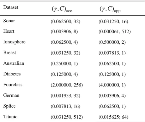
, running time and the ACVE under different sampling size.We take the parameter produced by APT under the sampling size c0.4n as the approximate optimal parameter and the parameter produced by the original kernel matrix as the accurate optimal model. Table III shows the comparison between accurate and approximate optimal parameters of different datasets, where the subscript “acc” and “app” are the abbreviation for accurate and approximate. We compare the solving time and the 5-fold cross validation accuracy between these two different optimal parameters. The results are shown in Table IV. We can find that the time for obtaining the
approximate optimal parameter is obviously less than that of the accurate optimal parameter and the time gap grows rapidly as the growth of dataset’s size. Nevertheless, the TSA between different optimal models are very close.
VI. CONCLUSION
In the core of SVM training lies a convex optimization problem which scales with O n( 3). But in many real-world applications, it is prohibitive to directly train SVM for every candidate parameter.
In this paper, we have presented and analyzed an algorithm APT which provides an approximate result of parameter tuning. We use a low dimension and low rank approximate kernel matrix generated by MoCIC to replace the original matrix in the inner-layer of APT. Because of the special structure of the approximate kernel
TABLE II.
OPTIMAL PARAMETERS, RUNNING TIME AND ACVE UNDER DIFFERENT SAMPLING SIZE.
Dataset Sampling size C Time(s) ACVE(%)
41 0.125000 2 64.8 29.8
Sonar 82 0.031250 16 132.9 16.2
123 0.062500 8 261.8 14.4
54 0.001953 4 181.2 19.3
Heart 108 0.000061 512 429.0 16.3
162 0.015625 2 961.1 14.4
70 0.500000 1 169.0 23.4
Ionosphere 140 0.500000 2 431.6 10.2
210 0.250000 1 1041.1 5.7
136 0.000977 1 660.0 3.2
Breast 272 0.007813 1 2334.8 2.5
408 0.003906 2 6394.2 2.3
138 0.001953 1 481.0 14.1
Australian 276 0.062500 1 1360.8 13.8
414 0.015625 16 3544.7 13.8
143 0.003906 4 561.3 31.4
Diabetes 286 0.125000 1 1480.1 24.0
429 0.062500 4 3762.3 23.0
172 0.062500 2 1479.2 28.9
Fourclass 344 4.000000 1 5493.5 7.2
516 4.000000 64 15952.8 0.2
200 0.125000 4 1099.1 27.3
German 400 0.003906 4 3540.2 25.8
600 0.007813 8 9824.7 24.7
200 0.500000 1 920.1 46.1
Splice 400 0.062500 1 3502.8 29.0
600 0.031250 2 10107.1 17.6
440 0.031250 1 5509.0 21.8
Titanic 880 0.015625 64 31215.1 21.8
matrix, parameter tuning algorithm could be conducted more efficiently. We make a time complexity comparison between the APT approximate algorithms and other parameter tuning algorithm. By experiments on 10 artificial and benchmark datasets, we verify the feasibility and the efficiency of APT. Experimental results show that the approximate parameter tuning approach is a sound and efficient parameter tuning framework.
ACKNOWLEDGMENT
The work was supported in part by the National Natural Science Foundation of China under grant No. 61170019 and the Natural Science Foundation of Tianjin under grant No. 11JCYBJC00700.
REFERENCES
[1] V. Vapnik, The Nature of Statistical Learning Theory.
New York, NY: Springer-Verlag, 1995.
[2] I. Guyon, A. Saffari, G. Dror, and G. Cawley, “Model selection: Beyond the bayesian/frequentist divide,” Journal of Machine Learning Research, vol. 11, pp. 61–87, 2010. [3] K. Duan, S. Keerthi, and A. Poo, “Evaluation of simple
performance measures for tuning SVM hyperparameters,”
Neurocomputing, vol. 51, pp. 41–59, 2003.
[4] C. Huang and C. Wang, “A GA-based feature selection and parameters optimization for support vector machines,”
Expert Systems with Applications, vol. 31, no. 2, pp. 231– 240, 2006.
[5] F. Friedrichs and C. Igel, “Evolutionary tuning of multiple SVM parameters,” Neurocomputing, vol. 64, pp. 107–117, 2005.
[6] V. Vapnik and O. Chapelle, “Bounds on error expectation for support vector machines,” Neural Computation, vol. 12, no. 9, pp. 2013–2036,2000.
[7] O. Chapelle, V. Vapnik, O. Bousquet, and S. Mukherjee, “Choosing multiple parameters for support vector machines,” Machine Learning, vol. 46, no. 1, pp. 131–159, 2002.
[8] Keerthi, S.S., “Efficient tuning of SVM hyperparameters using radius/margin bound and iterative algorithms,” IEEE Transactions on Neural Networks, vol. 13, no. 5, pp. 1225– 1229, 2002.
[9] Z. Xu, M. Dai, and D. Meng, “Fast and efficient strategies for model selection of Gaussian support vector machine,”
IEEE Transactions on Systems, Man, and Cybernetics, Part B: Cybernetics, vol. 39, no. 5, pp. 1292–1307, 2009. [10]L. Jia, S. Liao, and L. Ding, “Learning with uncertain
kernel matrix set,” Journal of Computer Science and Technology, vol. 25, no. 4, pp. 709–727, 2010.
[11]A. Frieze, R. Kannan, and S. Vempala, “Fast Monte-Carlo algorithms for finding low-rank approximations,” Journal of the ACM, vol. 51, no. 6, pp. 1025–1041, 2004.
[12]P. Drineas and M. Mahoney, “On the Nyström method for approximating a Gram matrix for improved kernel-based learning,” Journal of Machine Learning Research, vol. 6, pp. 2153–2175, 2005.
[13]S. Fine and K. Scheinberg, “Efficient SVM training using low-rank kernel representations,” Journal of Machine Learning Research, vol. 2, pp. 243–264, 2002.
[14]D. Achlioptas and F. McSherry, “Fast computation of low-rank matrix approximations,” Journal of the ACM, vol. 54, no. 2, pp. 1–19, 2007.
[15]G. Golub and C. Van Loan, Matrix Computations. Baltimore, MD: Johns Hopkins University Press, 1996. [16]P. Drineas, R. Kannan, and M. Mahoney, “Fast Monte
Carlo algorithms for matrices I: Approximating matrix multiplication,” SIAM Journal on Computing, vol. 36, no. 1, pp. 132–157, 2006.
[17]C. Williams and M. Seeger, “Using the nyström method to speed up kernel machines,” in Advances in Neural Information Processing Systems 13. Cambridge, MA: MIT Press, 2001, pp. 682–688.
[18]C. Williams, C. Rasmussen, A. Scwaighofer, and V. Tresp, “Observations on the nyström method for gaussian process prediction,” The Inference Group Website, Cavendish Laboratory, Cambridge University, 2002.
[19]C. Fowlkes, S. Belongie, F. Chung, and J. Malik, “Spectral grouping using the Nyström method,” IEEE Transactions on Pattern Analysis and Machine Intelligence, vol. 26, no. 2, pp. 214–225, 2004.
TABLE III.
ACCURATE OPTIMAL MODELS AND APPROXIMATE OPTIMAL MODELS
Dataset
acc
( , ) C ( , ) C app
Sonar (0.062500, 32) (0.031250, 16)
Heart (0.003906, 8) (0.000061, 512)
Ionosphere (0.062500, 4) (0.500000, 2)
Breast (0.031250, 32) (0.007813, 1)
Australian (0.250000, 1) (0.062500, 1)
Diabetes (0.125000, 4) (0.125000, 1)
Fourclass (2.000000, 256) (4.000000, 1)
German (0.001953, 32) (0.003906, 4)
Splice (0.007813, 16) (0.062500, 1)
Titanic (0.031250, 512) (0.015625; 64)
TABLE IV.
TIME AND TSA COMPARISION OF ACCURATE AND APPROXIMATE OPTIMAL MODELS.
Dataset Timeacc(s) Timeapp(s) TSAacc(%) TSAapp(%)
Sonar 522.2 132.9 87.1 86.2
Heart 1857.3 429.1 85.2 83.7
Ionosphere 2083.3 431.6 94.6 94.4
Breast 14423.5 2334.9 98.1 96.8
Australian 7690.4 1360.9 85.8 86.1
Diabetes 9784.4 1480.1 75.3 76.5
Fourclass 35839.8 5493.5 99.9 99.9
German 25902.0 3540.2 74.5 73.4
Splice 26961.2 3502.8 89.8 88.2
[20]T. Ho and E. Kleinberg, “Building projectable classifiers of arbitrary complexity,” in Pattern Recognition, 1996., Proceedings of the 13th International Conference on, vol. 2. IEEE, 1996, pp. 880–885.
[21]S. Liao and L. Jia, “Simultaneous tuning of hyperparameter and parameter for support vector machines,” in Proceedings of the 11th Pacific-Asia Conference on Knowledge Discovery and Data Mining (PAKDD 2007), Nanjing, China, 2007, pp. 162–172.
Chenhao Yang was born in Henan province, 1988. Sep 2006 to Jul 2010: TianJin University, Computer Science and Technology professional bachelor. Sep 2010 to now: TianJin University, Computer Science and Technology academic master. Mr Yang’s main research interests stochastic and random algorithm for support vector machines.
Lingzhong Ding was born in Inner Mongolia province, 1986. Sep 2005 to Jul 2009: TianJin University, Computer Science and Technology professional bachelor. Sep 2009 to now:
TianJin University, Computer Science and Technology PhD. Dr Ding’s main research interests include machine learning and model selection. He’s a student member of China Computer Federation.
Shizhong Liao was born in Mianyang Sichuan province, 1964. Sep 1981 to Jul 1985: Dalian University of Technology, Computer Science and Engineering, Computer Software, professional bachelor. Sep 1985 to Jun 1988: Jilin University, Computer Science, the artificial intelligence professional, master's degree. Sep 1994 to Jul 1997: Tsinghua University, Computer Science and Technology department, artificial intelligence professional, doctor.
He worked as professor in Liaoning Normal University from Jun 1988 to Jun 2003. From Jul 2003 until now, he is professor and PhD supervisor in TianJin University.