ISSN (e): 2250-3021, ISSN (p): 2278-8719
Vol. 08, Issue 7 (July. 2018), ||V (II) || PP 88-99
Simulation of Forecasting Performance Comparison of a Hybrid
Model Integrated By Binomial Smoothing and Bayesian Model
Averaging Techniques
Augustine D.Pwasong
,*, Caleb NanchenNimyel
b,Garba G. Naankang
ca*Department of Mathematics, University of Jos, P.M.B. 2084 Jos, Nigeria bDepartment of Computer Technology, Plateau State Polytechnic Barkin-ladi,, Nigeria c
Department of Computer Technology, Plateau State Polytechnic Barkin-ladi,, Nigeria Corresponding Author: Augustine D.Pwasong
Abstract:
Inthis study, a hybrid JPSN-AR model is proposed based on binomial smoothing (BS) and Bayesian model averaging (BMA)techniques. The aim is to determine the combination technique that produced the best forecasting performance for the proposed hybrid model. The forecasting performance measurements employed to ascertain the foregoing assertion are the mean absolute percentage error (MAPE) and the root mean square error (RMSE). The results revealed that the best performance of the proposed hybrid model was achieved through the combination of the Jordan pi-sigma neural (JPSN) network model and an autoregressive(AR) time series model by the Bayesian model averaging (BMA) technique. Although the combination that produced the hybrid model made by the binomial smoothing technique also produced good forecasting performance by the hybrid model, but the combination technique with the Bayesian model averaging(BMA) technique puts the proposed hybrid model at its best. Simulations in this study are made possible by using MATLABsoftware version 8.03Keywords:
Binomial smoothing; ARIMA; Combination;MAPE, RMSE; Forecasting, AR; Bayesian model averaging; Stationary; JPSN; Neural nets; Nonlinear; Linear and Performance--- Date of Submission: 28-06-2018 Date of acceptance: 13-07-2018 --- ---
I.
INTRODUCTION
In this study, we propose a hybrid method to time series forecasting using both the Jordan pi - sigma neural network (JPSN)and autoregressive (AR) model based on Bayesian Model Averaging (BMA) and Binomial Smoothing (BS)techniques in time series data processing, which is called the hybrid JPSN-AR model. In the hybrid JPSN – ARtechnique, a neural network model known as the Jordan pi-sigma neural network
(JPSN) is combining with an autoregressive model. The combination techniques employed here are the Bayesian Model Averaging technique (BMA) and the Binomial Smoothing (BS) technique. The AR model used in the proposed hybrid model is the Box-Jenkins methodology also known as the ARIMA model, i.e. autoregressive integrated moving average model. The performance of the hybrid JPSN-AR model based on the
BMA combination technique is compared with its performance based on the BS combination technique in order to determine the combination technique that provides the hybrid JPSN-AR model with the best forecasting performance.
Latiflogu[3] proposed a forecasting technique for nonstationary and nonlinearhydrological time series data points grounded on singular spectrum analysis (SSA)and artificial neural networks (ANN). They employed
SSA to decompose the stream flow data points into its independent mechanism. In their model, the decomposed stream flow data points, metamorphosed into independent mechanism characterizingthe trend as well as oscillatory pattern of hydrological data points and serves as the exact target variable in the neural network that will follow, to make forecast for 1 month ahead stream flow time series data points. The hybrid ANN-SSA model takes thebenefit of the distinctive strength of ANN and SSA in nonlinear and linear modeling. The advantages of such approachesseem to be significantparticularly when dealing with non-stationary series: non-stationary nonlinear component using neural network model and the residual is a stationary linear component which can be modeled by SSAmodel. They alsoemployed the mean square errors (MSE), mean absolute errors (MAE) and correlation coefficient (R) statistics to appraise the forecasting capability of the anticipated technique. The outcome of their findings revealed how the hybrid SSA−ANN model became a suitable technique for hydrological data set forecasting. They also compared the forecasting performance results of the hybrid
SSA−ANN with the forecasting performance of standalone ANN model and the outcome of the comparison revealed that the hybrid SSA−ANN outperforms the single ANN model for 1 month ahead of forecasting of stream flow time series data points. Furthermore, they validate the practical efficacy of the proposed hybrid
SSA−ANN model and standalone ANN models from 1 to 6 months forward for forecasting of hydrological time series data points.
Dong and Liu asserts that ANN models and ARIMAmodels constitute a veritable tool for modeling and forecasting nonlinear time series in view of the over-fitting problem which is possible to happen in neural network models. Since the parameters of neural networks are only lambda values that need to be trained and the Bayesian Model Averaging technique as well as the Binomial Smoothing technique are effective in time series data processing [4].
The outstanding segments of this study are structured asfollows. In sectionII, ANN modelling,Bayesian Model Averaging preprocessing methods and Binomial Smoothing preprocessing methods to form a hybrid forecasting model as well as ARmodeling methods to time series forecasting is reviewed. The proposed hybrid
JPSN –ARmethodology is presented in Section III. In section IV, experimental results from real time series data are explained.Concluding remarks are reported in Section V.
II.
METHODS IN FORECASTING TIME SERIES DATA
A. Bayesian Model Averaging (BMA)Technique
Raftery et al [5] affirmed that a combination technique that merges the forecastsof two or more forecasting models is known as the Bayesian Model Averaging (BMA)technique. He declared that the BMA
amalgamation technique generates a consensusweighted forecast on the basis of weighting the variances of any distinct model orweighting the prediction mean square errors of any lone model. In order to maintainthe
BMAtechnique employed in this study, one may advance as tag along. Supposethat M = {M1,M2} signifies the
class of two schemes which is being considered inthis paper such that Δ is a measure of engrossment referred to as the target input orvariable, then the latter classification known as the posterior distribution of Δ given thedata
Gis:
Pr(Δ|G) = Pr(Δ|M1,G)P1(M1|G)+Pr(Δ|M2,G)P2(M2|G) (1)
Equation (1) is the mean of the posterior distributions in every model weighted by the resultant posterior model probabilities. This is called the Bayesian Model Averaging (BMA). In equation (1) the posterior probability of model Mkwhere k=1,2 is specified as:
21
k
l r l r l k r k r
k r
M
P
M
G
P
M
P
M
G
P
G
M
P
(2)Where
k
r
k k
r k k
k rG
M
P
G
M
P
M
d
P
,
(3)is the marginal likelihood of model Mk, θk is the vector of parameters of model Mk,
P
r
kM
k
is the priordensity of θk under model
M
k,
P
r
G
k,
M
k
is the likelihood, andP
r
M
k is the prior probability thatMkis the exact model. All probabilities are totally restricted on M, the set of the two models being entertained in
weights ωk k = 1,2 is defined by ωk=p(G|Mk) such that Σωk= 1. There exist some striking characteristics of the
BMA method. The BMA technique
is predictively and statistically strong, such that it became the reason for which it is used here as a nonlinear scheme in the modeling and forecasting methodology. Also, the BMA technique allocates high weights to models that are superior in performance established on the chances of presenting a model. The BMA
technique possesses a numerical variation which is less than the variances of some lone models since it handles effectively any inter-model-variance and intra-model-variance.
Suppose 1
S
and 2
S
are forecasts completed by models M1 and M2respectively, then 2 1
and
22 are respectively variances of M1 and M2such that their expectation and variance is defined in the followingequations. 2 1 1 1 2
1
,
,
S
S
G
S
S
S
E
(4)and 2 2 2 2 1 1 2 2 2 1 1 2 2 2 2 2 1 1 1 1 2
1
,
,
S
S
S
S
S
S
G
S
S
S
Var
(5)B. Binomial Smoothing (BS) Technique
Dong and Liu are of the view that with ANNs, the nonlinear model procedure must be estimated from the time series data. Hence, the over-fitting problem is expected to occur in neural network models. That is, the network fits the training data exactly, but has insufficient generalization
capability for out of sample data [4]. Marchand and Marmet asserts that smoothing by long least-squares polynomial (LSP)sequences points to phase reversals and overshoots that may be objectionable in some applications[6]. They however explained that the binomial smoothing technique whose smoothing structure is well defined by the binomial coefficients can overcome the problems of overshoots and phase reversals.
Zheng and Zhong [7] asserts that every three-point binomial smoothing
z
k of an n-point data sequence
y
k can be performed as follows:
2
,...,
2
,...,
2
,...,
2
,...,
2
1 2 1 2 1 1 1 2 1 1 k k k n n n k k kw
w
z
w
w
z
y
y
w
y
y
w
y
y
w
2
,...,
2
2
2
2
2
1 2 1 2 1 1 1 1
n n n k k k k k k kz
z
z
x
x
x
y
y
y
y
Finally,
z
k
y
1
w
1
2
and
w
n1
y
n
2
.This preserves the end points to remain static and evades growing end effects. Also, this approach is faster than employinglengthier binomial structures directly or LSPsmoothing. The definition of a three-point binomial smoothing structure is given bythe binomial coefficients as
22
1
,
2
,
1
.A binomial smoothing structure of the points of order n+1 is given by:
nn
n
C
k
n
C
n
C
n
C
,
0
,
,
1
,...,
,
,...,
,
2
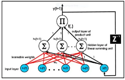
C. The Jordan Pi-Sigma Neural (JPSN) Network
shown in Figure 1.In Figure 1, x(t) represents the input nodes at tth time, ωkj is the trainable weights, hk(t+1) is
the summing unit, y(t+1) is the output at time (t+1),y(t) is the output at time t and f(.) is the activation function.Weights from the input layers x(t) to the summing units layer are tunable, while weights between the summing unit layers and the output layer are fixed to 1. The tuned weights are employed for network testing to determine the extent of fitness the network model simplifies on undetected data.𝑧−1 denotes time delay
operation.
Suppose the quantity of outer inputs to the network isQand the quantity of the output be 1. Let xq(t) be the q–thouter input to the network at time t. The general input at time t is the
Figure 1: Architectural Design of the Jordan Pi-Sigma Neural (JPSN) Network
Concatenation of y(t) andxk(t) wherek =1,...,Q,and is referred to as z(t) where:
2
1
1
1
Q
k
if
t
y
Q
k
if
Q
k
if
t
x
t
z
k k
k
For the time being, weights from z(t) to the summing unit are set to 1 in order to decrease the Complexity of the network. The JPSN pools the properties of both Pi-Sigma Neural Network and Jordan Recurrent Neural Network, hence the name „Jordan Pi-Sigma Neural Network‟. The supervised learning employed in JPSN can be resolved with the standard backpropagation(BP) gradient descent algorithm, through the recurrent link from outputlayer back to the input layer nodes[9]. Meanwhile, identical weights are employed for all networks, the learning algorithm starts by resetting the weights to aninsignificantarbitrary value before training the weights. The JPSN is conveniently trained in which the errors formed are computed and the general error function E of the JPSN is given by
t
d
j
t
y
j
t
j
(6)where
d
j
t
denotes the target output at timet
1
. At each timet
1
, the output of eachy
j
t
is determinedand the error
j
t
is computed as the variation between the actual values expected from each unit I and the1. Calculate the output.
K L Lt
h
f
t
y
1 (7)
t
h
L can be computed as
q q q q q Lq q L q L q LqL
t
x
y
t
z
t
h
1
1
1
1
1
Where
h
L
t
signifies the activation of the L unit at time t, and y(t) is the previousnetwork output. The unit‟s transfer function f sigmoid activation function is bounded by the output range of [0,1]2. Compute the output error at time (t) using standard Mean Squared Error (MSE) byminimizing the following index:
nHi
k i i H
k
y
z
n
E
1 21
(8)Where
z
ikdenotes the output of the kthnode sequel to the ith data, andn
His thequantity of training sets. This stage is accomplishedcontinually for all nodes on the current layer.3. Employ the BP gradient descent algorithm to compute the weight changes by
k q
j ji j
h
x
1
(9)where
h
jiis the output of summing unit and
is the learning rate.4. Bring up to date the weight:
i i i
(10)5. To fast-track the convergence of the error in the learning process, the momentum term,
is added into Equation 8. At this moment, the values of the weight for the interconnection on neurons are computed and can be numerically expressed asi i
i
(11) where the value of
is a user-selected positive constant
0
1
6. The JPSN algorithm is ended when all the ending conditions (training error, maximum epoch and early stopping) are fulfilled, otherwise, repeat step 1)
D. the Autoregressive (AR) time series model
For a stationary time series, the autoregressive(AR) time series model transmits the future value to past and present values in a linear manner. An autoregressive process of order p is given by
t p t p t t
t
y
y
y
y
1 1
2 2
....
(12)where
i
i
1
,
2
,...,
p
are the autoregressive parameters, μis the mean of the series and
t is a random process witha mean of zero and a constant variance of
2.sufficiency. Quite a lot of diagnosticstatistics and plots of the residuals can be employed to scrutinizethe goodness of fit of the model to the time series data.
An ARIMA model is written as ARIMA(p,d,q) where the order of autoregressive termsis given by p,the number of times the non-stationary time series requires to be differenceto make it stationary is given by d and the order of the moving average partof the ARIMA model is given by q which is the number of lagged forecast errors. TheARIMA(p,d,q) process is generally written as
t
td
y
1
0
(13)Where𝜃0is an intercept term.Akpanta and Okorie [10] employed Box-Jenkins techniques in modelling
and forecasting Nigeria crude oil prices from 1982 to2013. To make the time series observations stationary, they used first order differencingwhich is a condition that permits the use of the univariate Box- Jenkins modelling technique. They also observed that the plots of the time series data, the autocorrelation (ACF)and the partial autocorrelation function (PACF)of the first order difference suggested ARIMA(6,1,7) which was characterizedby a lot of model parameters that were redundant as a result of which they fitted anARIMA(2,1,2). This led to a reduced and parsimonious model. They further compared the outcomes of fitting ARIMA(2,1,2) to the time series observations with theoutcomes of fitting ARIMA(6,1,7) to the time series data points such that they usedARIMA(2,1,2) to make forecasts because it performed better than ARIMA(6,1,7).
III.
THE METHODOLOGY OF THE HYBRID FORECASTING MODEL
Given thattime series observations are not often pure linear or nonlinear, we therefore combinedANN
model with AR model such that complex autocorrelation patterns in the data can indeed be modelledcorrectly. Furthermore, since real- world time series data possesses changing patterns, employing the hybrid approachcan decrease the model ambiguity which usually occurs ininferential statistics and time series forecasting [11].It is appropriate to consider a time series in this study to be a function of a linear autocorrelationstructure and a nonlinear component. The proposed hybrid model ℎ𝑡is represented asfollows:
t t t
a
b
h
(14)where 𝑎𝑡 denotes the nonlinear part of the hybrid time series model and𝑏𝑡denotes thelinear part. The
two components 𝑎𝑡 and 𝑏𝑡must be estimated from the time series data. In this study, the proposed hybrid J
PSN-AR model whose nonlinear component is the neural network part of the modelmodelled by JPSN is integrated with the linear component of the model being a time series autoregressive model modelled by ARIMA using binomial smoothing. Also, the two components of the proposed hybrid JPSN-AR model are integrated using the
BMA combination technique after which the forecasting performance of the hybrid model using BS technique and BMA technique is compared to determine which combination technique produced the best forecasting performance for the proposed hybrid JPSN-AR model.
A. The hybrid JPSN-AR model integrated by binomial smoothing (BS)preprocessing
In this section, the proposed hybrid JPSN-AR model combined the nonlinear component (JPSN) with the linear component (AR) using binomial smoothing. The time series data sets are first smoothed by BS
technique and the smoothed data sets are modeled by JPS neural network. This process will lead to the removal of the stationary nonlinear component of the series. The residuals emanating from the removed non-stationary nonlinear component are now non-stationary linear and are modeled by AR model. Residuals are important indiagnosis of the sufficiency of linear models. A linear modelis not sufficient if there are still linear correlation structuresleft in the residuals. Lastly, the predicted components from both JPSNnetwork and AR
model are integrated to acquire the overall prediction. The outcomepoints out that the over-fitting problem can be alleviated by means of JPS neural network based on binomial smoothing in the time series data. Hence, the combined forecast is
t t t
a
b
h
(15)B. The hybridJPSN-AR model integrated by Bayesian model averaging (BMA) preprocessing
In this section, the proposed hybrid JPSP- ARmethod is made possible by combining the JPS neural network method and the ARIMA time series method by means of the BMA technique. This combination method involves five stepsof calculations: (i) data are modelled by the ARIMA technique first; (ii) the residuals of the
The underlying principle behind this hybrid JPSN – ARmethod is that linear relations among
input and output variables are modelled by the ARIMA method, while nonlinearrelations amid input and output variables are modelled by the nonlinear JPSNnetwork. For the period of neural network training steps, both the least MSE criterion and the leastMAE criterion are employed to conserve the optimization results for non-Gaussian distributeddata. The Bayesian model averaging (BMA) technique is a weighted average method that permits weighting factors to be assigned based on the forecasting performances of the twoseparately trained neural networks.
C. The Root Mean Square Error (RMSE) and Mean Absolute Percentage Error (MAPE)
The root mean square error (RMSE) and mean absolute percentage error (MAPE) are methods of measuring a time series model‟s accuracy. In this study we examine the forecasting accuracy by
calculating these two different evaluation statistics, i.e. the RMSE and MAPE. The mean squared error
(MSE) is described as estimate of variation of errors in forecasting. Apparently, the variation of errors in statistics ought to be small. The MSE is dependent on balance estimates of accurate predictions, that is, its estimates arearticulated in requisites of its unique components of measurement [12]. The following equation is applicable in obtaining the MSE.
n i t tF
A
n
MSE
1 21
(16)where 𝐴𝑡is the actual output and𝐹𝑡is the predicted output and n is the quantity ofterms in the class of
data.Also, they declared the root mean square error (RMSE) as an estimate of the standard degree of error. The square root of the mean is taken in view of the fact that the errors are squared prior to the averaging, such that the RMSE presents a moderately lofty weight to huge errors. This implies that the RMSE is mainly functional as soon as huge errors are predominantly unwanted. The RMSE is expressed by the equation below.
n i t tF
A
n
RMSE
1 21
(17)In another development Saigal and Mehrotra [12] also defined the mean absolute error (MAE) as an estimate of the complete quantity of the difference between the predictable observations and the original observations simultaneously such that the negative observations do not cancel the positive observations. The
MAE is however obtained after averaging the stated observations. The MAE is express by the equation below.
n i t tF
A
n
MAE
11
(18)where 𝐴𝑡 is the preferred output and 𝐹𝑡is the predicted output and n is the quantity of terms in the class
of data.
Tayman and Swanson [13] asserts that the mean absolute percentage error (MAPE) is the MAE divided by the preferred output and multiplying by 100 makes it a percentage error. It usually expresses accuracy as a percentage. The MAPE is defined by the formula below.
n i t t tA
F
A
n
MAPE
1100
1
(19)where 𝐴𝑡 is the preferred output and 𝐹𝑡is the predicted output and n is the quantity of terms in the class of data.
IV.
PREPROCESSING AND DECOMPOSITION OF REAL TIME SERIES DATA
A. Daily Time Series Data and Increments
model and prediction on the basis of the built model implies to forecast sequel to the developed model. The hybrid model is made to create 1728 predictions.
The daily time series recordings from a chemical platform is represented in Figure 2 which illustrates the entire picture of 3086 time series sample data for the study. The mean of the data series is 45.32. The median is 26; while the mode is 1.10 and the variance is 9.4636e+03. The maximum value of the data series is 2630 and the minimum value is 0.10. Figure 2 is plotted by the MATLAB software version 8.03
Figure 2: Time Series Recordings from a Chemical Platform
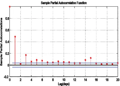
Figure 4: Sample PACF of the Chemical Platform Series
Figure 3 is the picture of the sample autocorrelation function (ACF) of the daily time series recordings from a chemical platform with 95% confidence bound. This picture is graphed by enacting the autocorr(xdata)
command in MATLAB. Also, Figure 4 shows the picture of the sample partial autocorrelation function of the daily time series recordings from a chemical platform with 95% confidence bound. The picture is graphed by enacting the parcorr(xdata) command in MATLAB. Figures 3 and 4 revealed that the daily time series recordings from a chemical platform are autocorrelated and partially autocorrelated.
In this study, we considered one out of several ways to form an increment series. An increment series here is referred to as the log difference series of the original time series data. An increment series is formed by differencing the original daily time series data in log. Suppose 𝑦𝑡 is the original time series data, then 𝑍𝑡 =
𝑙𝑜𝑔 𝑌𝑡 − 𝑙𝑜𝑔 𝑌𝑡−1 is the increment series and since it is obtained by taking the differenceof the logarithms of
the original daily time series data, it is also called log difference series. Figure 5 illustrates the picture of the daily log difference time series recordings from a chemical platform. The MATLAB commands mean(zdata), median(zdata), max(zdata) and var(zdata) is implemented to determine the mean, median, maximum value and variance respectively for the log difference series. Hence, the mean value=1.2538e0.04, the median value = -0.0029, the maximum value = 2.6902 and the variance = 1.1583. The log difference series has a smaller variance than the original series;therefore, we will proceed with the log difference for further analysis in this paper. An examination of trend stationary enacted by the Augmented Dickey-Fuller (ADF) tests (trend stationary t test, AR
. Figure 5: Log Difference Series of the Chemical Platform Series
Figure 6 is the picture of the sample autocorrelation function of the daily log difference time series recordings from a chemical platform.
Figure 6: Sample ACF Function of the Log Difference of the Chemical Platform Series
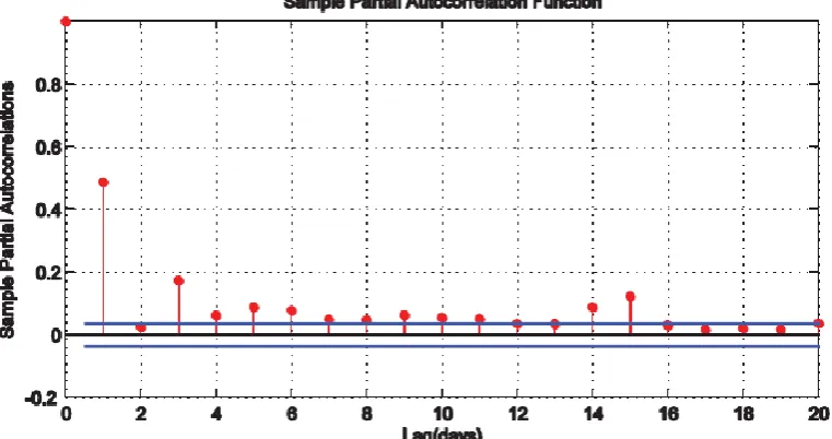
Figure 7: Sample PACF of the Log Difference of the Chemical Platform Series
Logarithm of the time series also put forward an order 2 moving average (MA(2)) model for the log difference series, as one can observe from the plots of the autocorrelation and partial autocorrelation, it is only the first two sample autocorrelation functions are roughly significant, and all partial autocorrelation functions diminishes rapidly ( approximately geometrical decay). Normally, an MA(q) model possessed structures of autocorrelations cutting off after lag q and partial autocorrelations tailing off.
Since the autocorrelations and partial autocorrelations plots of the increment series, that is, log difference series evidently suggested MA(2) models, one will notice that the log difference series are better in modelling and forecasting than the original chemical platform series. Also, the variance of the log difference series is smaller than the variance of the original time series data. Strictly speaking, working on the log difference series gives three solid benefits. Firstly, since the variance of the log difference series is smaller than the variance of the original series, it will lead to smaller mean square error for the log difference than for the original time series. Secondly, an obvious moving average (MA(2)) is realizable as explained above. Thirdly, the original time series data is an autocorrelated series while an increment series of the log difference collection is almost an independent and normally distributed series. Hypothetically, employing an independently and normally distributed series is easier than otherwise.
B. Results
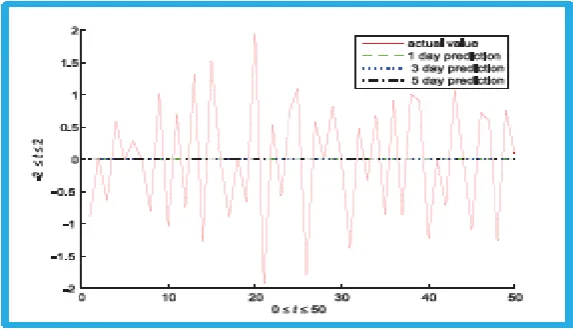
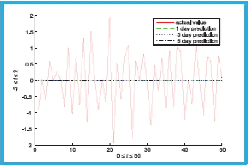
In this study, neural network models are built using the JPS neural network. Only the 1 day ahead prediction, 3 days ahead prediction and 5 days ahead prediction produced by the hybrid JPSN-AR model based on binomial smoothing and Bayesian model averaging techniques isconsidered. Four inputs are used in neural model.Figure 8 gives the actual values and the forecast values for the hybrid JPSN-AR model based on binomial smoothing using the log difference series of the chemical platform series.
Figure 9 gives the actual values and the forecast values for the hybrid JPSN-AR model based on binomial smoothing using the log difference series of the chemical platform series. The predicted
Figure 9: Hybrid JPSN-AR prediction based on BMA technique
Values for 1 day, 3 days and 5 days ahead prediction for the log difference of the chemical platform series are overlapping and lying at the point 0 which is the centre of the graph. This trend indicates that the predicted values are stationary thereby resulting in accurate forecast values produced by the proposed hybrid
JPSN-AR method based on the BMA technique as it is illustrated in Figure 9. The results also revealed that the hybrid method basedon BMAtechnique can relieve the over-fitting setback and can be employed for forecasting time series as well capture all ofthe patterns in the data. The foregoing claim has confirmed the assertion made in sections II(A) andIV(A) thatthe original time series data is an autocorrelated series while an increment series of the log difference collection is almost an independent and normally distributed series and it has a smaller variance than the original series. Also, the predicted values for 1 day, 3 days and 5 days ahead prediction for the log difference of the chemical platform series are almost overlapping and lying very near to the abscissa of the curve which is the line 0. This trend also indicates that the predicted values are stationary thereby resulting in accurate forecast values produced by the proposed hybrid JPSN-AR method based on the BS technique as it is illustrated in Figure 8. However, the performance of the hybrid JPSR-AR method based on the BMA technique is better than its performance based on the BS technique since the predicted values are greatly stationary thereby resulting in greater accurate forecast values than those produced by the hybrid model based on the BS technique. This may be attributed to fact that the hybrid method based on BS technique may not capture all of the data patterns in the log difference series of the chemical platform series. This assertion is further proclaimed in Table 1 where the overall forecasting errors significantly reduced the MAPE and RMSE of the hybrid method based on
BMA technique over the hybrid method based on BS technique.
Table 1: The Forecasting Performance Results of the Hybrid JPSN-AR Model
Hybrid JPSR-AR
model based on BS technique
MAPE RMSE Hybrid JPSR-AR model
Based on BMA technique
MAPE RMSE
Prediction 1 day ahead 0.0463 0.01038 Prediction 1 day ahead 0.6099 0.4517
Prediction 3 days
ahead
0.0463 0.01038 Prediction 3 days ahead 0.5999 0.4401
Prediction 5 days
ahead
0.0617 0.01026 Prediction 5 days ahead 0.6199 0.4517
V.
CONCLUSION AND RECOMMENDATION
The proposed hybrid JPSN-AR model based binomial smoothing and the Bayesian average modelling techniques, is very robust and consistent. They all have very stable forecasting results
for a very short data length. Their forecasting performances are comparable to and to some extenthealthier than standalone neural networks and standalone time series models such as feedforward neural networks (FNN) models, recurrent neural network (RNN) models, ARIMA models, etc. They have slightly better
MAPE and RMSE performances than the aforementioned standalone models. However, the proposed hybrid
International organization of Scientific Research
99 | P a g e
We have restricted our study for one data series of the chemical platform series. Further studies are suggested to cover two or more data series can have improved forecasting pictures. Indeed, when covering two or more data series, forecasting models mayturn out to besomewhat complex. For example, a time series
ARmodel becomes a VAR (vector autoregressive) model.
REFERENCES
[1]. Cochrane, J. H. (2005). Time series for macroeconomics and finance, Manuscript,University of Chicago
[2]. G. Peter Zhang, Time series forecasting using a hybrid ARIMA and neuralnetwork model,
Neurocomputing, vol. 50, pp. 159 - 175, 2003.World Academy of Science, Engin
[3]. Latifo˘glu, L., Ki¸si, Ö. and Latifo˘glu, F. (2015). Importance of hybrid models for forecastingof hydrological variable, Neural Computing and Applications 26(7): 1669–1680
[4]. C.J. Dong and Z. YLiu, A simulation study of artificial neural networksfor nonlinear time-series forecasting ,Computers & Operations Research,vol. 28, pp. 381–396, 2001
[5]. Raftery, A. E., Madigan, D. and Hoeting, J. A. (1997). Bayesian model averagingfor linear regression models, Journal of the American Statistical Association92(437): 179–191
[6]. P. Marchand and L. Marmet, Binomial smoothing filter: A way to avoid some pitfalls of least-squares polynomial smoothing, Review of ScientificInstruments, vol. 54, pp. 1034 - 1041, 1983.
[7]. Fengxia Zheng and Shouming Zhong (2011).Time series forecasting using a hybrid RBF neuralnetwork
and AR model based on binomialsmoothing. World Academy of Science, Engineering and Technology Vol:5, pp. 1177-1181
[8]. Ghazali, R.: Hussain, A. J. &Liatsis, P. (2011). Dynamic Ridge Polynomial Neural Network:Forecasting the univariate non-stationary and stationary trading signals. Elsevier:Expert Systems with Applications. 38, pp. 3765-3776.
[9]. Rumelhart, D. E.: Hinton, G. E. & Williams, R. J. (1986). Learning Representations by Back-Propagating Errors. Nature, 323 (9), pp. 533-536.
[10]. Akpanta, A. and Okorie, I. (2014). Application of box-Jenkins techniques in modellingand forecasting Nigeria crude oil prices, International Journal of Statisticsand Applications 4(6): 283–291.
[11]. C. Chatfield, Model uncertainty and forecast accuracy, J. Forecasting,vol. 15 pp. 495–508, 1996.
[12]. Saigal, S. and Mehrotra, D. (2012). Performance comparison of time series data usingpredictive data mining techniques, Advances in Information Mining 4(1): 57–66.
[13]. Tayman, J. and Swanson, D. A. (1999). On the validity of map as a measure ofpopulation forecast accuracy, Population Research and Policy Review 18(4): 299–322.