A Stochastic Approach to Predicting Performance of Web Service Composition

(1)

A Stochastic Approach to Predicting Performance

of Web Service Composition

*

Yuxiang Dong

School of computer science, Chongqing University, Chongqing, China Email: [email protected]

Yunni Xia﹩ and Qingsheng Zhu and Ruilong Yang School of computer science, Chongqing University, Chongqing, China

Abstract—In this paper, we propose an analytical approach to predict the performance of web service composition built on BPEL. The approach first translates web service composition specification into Stochastic Petri Nets. From the SPN model and its corresponding continuous-time Markov chain, we derive the analytical performance estimates of process-completion-time. In the case study, we also use computer simulation techniques to validate our analytical model.

Index Terms—service composition, performance, stochastic Petri net

I. INTRODUCTION

In recent years, many research efforts have been made in the web services composition and various composition languages have been proposed, including BPEL [1], BPML or ebXML. An important research issue is how to assess the degree of trustworthiness. Although many efforts have been made to insure functional correctness of composed services through formal verification techniques [2, 3, 4, 5, 6], prediction of nonfunctional and quantitative characteristics such as performance, reliability, availability is less studied. Although one can quantitatively measure those metrics through running or testing real systems, measurement-based approaches can only apply to those available service compositions (at least their executable prototypes) but not services still at design phase. Moreover, measurement-based approaches can be costly and time-consuming. Therefore, analytical approaches are more preferable. Analytical approaches aim at taking parameters (can be specified by service providers or evaluated based on historical records) of service components as input and automatically generating quantitative estimates.

In this paper, we propose an analytical approach to predict performance (in terms of process-normal-completion-time) of composite web services built on BPEL employing stochastic Petri net as the intermediate model. Through analyzing the homogeneous continuous

Markov chain derived from the stochastic Petri net, we can calculate the process-normal-completion-time analytically. We also employ the Montecarlo simulation to obtain experimental results of process completion-time and show theoretical estimation is validated by simulative results.

II. PRELIMINARIES

A. BPEL

A composite service in BPEL is described in terms of a process. Each element in the process is called an activity. BPEL provides two kinds of activities: primitive activities and structured activities. Primitive activities perform simple operations such as receive, reply, invoke, assign, throw, terminate, wait and empty. A structured activity is used to define the order on the primitive activities. It can be nested with other structured activities. The set of structured activities includes: sequence, flow, while, pick and scope. Structured activities can be nested. Given a set of activities contained within the same flow, the execution order can further be controlled through links. A link has a source activity and a target activity, the target activity may only start when the source activity has ended. With links, control dependencies between concurrent activities can be expressed.

B. Stochastic Petri net

Petri Nets is a tool used for modeling and analysis of complex system with behavioral patterns such as concurrency, synchronization and conflict. Original Petri net does not care the concept of time and was extended into various types of timed/stochastic Petri net. We base our research on stochastic Petri nets (GSPN):

Definition: A GSPN is a 5-tuple (P, T, F, M0,

λ

):

1. P={p1 , p2…pn} is a finite set of places

2. T is a finite set of transitions partitioned into two subsets:

TI(immediate) and TD(timed) transitions

3.

λ

: TD →real is a function identifying firing rate of each timed transition

4. F

⊆

(P * T)

∪

(T*P) is a finite set of directed arcs * Supported by the national 863 plans projects of China under grant

(2)

5. M0 is an initial marking

Note that, for modeling and performance prediction of real-world service compositions, firing rate of a certain task can often be specified by service providers or evaluated by means of averaging execution durations of historical records

i

1 (

)

Mean historical execution durations of td

i

td

λ

=

(1)

III. MAPPINGBPELINTOGSPN

A. Mapping of primitive activity

We start the mapping with the primitive activity where mapping rule is illustrated in Fig.1. A primitive activity (like, for example, invoke, receive and reply) does not contain any other activity. A primitive activity can have a join condition, a join-fault setting, a number of sources and a number of targets. In Fig.1, the body of the activity is illustrated by a rectangle. All input signals and conditions are modeled by places on the life border of the rectangular area while output ones on the right border. Places and transitions in the rectangular area capture internal states and state-changes.

Each primitive activity has the optional containers <sources> and <targets>, which contain collections of <source> and <target> elements respectively. These elements are used to establish synchronization relationships through a <link>. An activity can declare itself to be the source of one or more links by including one or more <source> elements. Similarly, an activity can declare itself to be the target of one or more links by including one or more <target> elements. Take Fig.1 for example, two links namely LINKa and LINKb are

introduced to establish dependence into and from the primitive activity, where LINKa is a incoming link

connecting a source of another activity to a target of the primitive activity while LINKb is a outgoing link

connecting a source of the primitive activity to a target of another activity. Timed transitions in links are used express delay of signal transmission. The targets (can be absent) are the incoming links that need to be examined before this activity can start. A target can have either a positive or a negative status. A token in the true target place (TTi) indicates the positive status while a token in

the false target place (TFi) indicates negative status.

Outgoing sources are similarly modeled through TSi and

TFi places. The join condition (evaluated to true if

absent) is a Boolean expression over targets, which is mapped onto a Boolean net [8]. For instance, the primitive activity in Fig.1 has two incoming targets and its join condition requires that a join success is achieved only if both targets are positive. Consequently, a boolean net (illustrated in the double-lined-parallelogram) is used to express the join condition where the join success (place JS) is marked only if both place TT1 and place TT2 each

contain a token.

Fig.1 Mapping of a primitive activity

The timed transition X denotes the actual execution of the activity which can only be started if the join condition evaluates to true. The SJF place is used to model the

suppressJoinFailure condition where a token in this

place indicates suppressJoinFailure="yes". In this case, the completed place is marked as if the activity encounters no join failure and outgoing sources are all set to negative. Otherwise, a fault is thrown through generating a token into the fault place and outgoing sources are all set to negative. An inhibition arc is also used to prevent place JF from generating fault when the condition suppressJoinFailure="yes" is imposed. Note that, to prevent arcs from crossing and simplify the illustration, dashed-bordered places are actually copies of the solid-bordered place and they are merged for semantic interpretation. The graphical simplification technique is also applied to other illustrations later on.

The normal control flow is captured by the token movement on the path started →enable→finished→ completed. When the normal control flow is successfully accomplished, output source signals (can be absent) is also generated (if the activity does have outgoing links). Every source signal can be either set to true (place TSi) or

false (place FSi) at runtime according to the transition

condition (evaluated to true if absent). Therefore, immediate transitions TCTi (transition condition

evaluated to true) and TCFi (evaluated to false) are used

to capture the nondeterministic generation of source signals.

The to_stop place is used to model the control interface of stopping the activity when faults occur. When to_stop contains a token, inhibition arcs from that place stops normal control flow and the status of the activity is changed to stopped (by generating a token into the stopped place).

Another important part of the mapping is the

dead-path-elimination (PDE for short). A dead path comes

(3)

B. Mapping of scope and handlers

The <scope> activity is WS-BPEL's most complex one which not only embeds an activity, but can also contain event, fault, compensation, and termination handlers (newly introduced in WS-BPEL 2.0). The mapping rule is given in Fig.2. Similar to Fig.1, input signals and conditions are represented by places on the left border while output ones on the right. Also, four places on the upper border are used to indicate the existence of fault handler, event handler, compensation handler and termination handler. Besides output interfaces for completion, fault and stopping indication, a pair of complementary places (snapshot and no_snapshot) are used to indicate whether fault has occurred. Moreover, the compensated place is also on the output border to indicate whether the scope has been compensated.

To have a clear view of interdependence among inner constructs, the scope is divided into five parts by dashed lines. The leftmost part captures the main activity (activity A1, may be primitive or structural) and its

control flow. Note that, A1 may have links if it is

primitive but links are not illustrated because they are not part of scope itself. When any fault happens (for instance a join failure fault), the place fault1 is marked. If a fault

handler is available (indicated by a token in place

FH_available), the token in fault1 is moved away and

place to_stop1 will be marked to stop the execution of A1.

On the other hand, if no fault handler is available, the token in fault1 is moved into fault_s, meaning the fault is

upgraded into a scope-level fault which can not be handled by the scope itself and is requiring fault-handling from parent scopes.

When the status of A1 is changed to stopped, the

execution of fault-handler is activated. The main activity of the handler, FH (may be primitive or structural) is enabled if it matches the fault type, otherwise it is skipped and fault_s is marked indicating a scope-level fault is generated. When the execution of FH is completed, not only place completed_FH but also completed1 are marked, to indicate the fault is

successfully handled. FH itself can have fault and its fault is treated as scope-level fault. Its fault is supposed to be handled by a fault handler in parent scopes and place to stop_s will be marked for fault handling.

When a successful completion of A1 is achieved, the

scope-level place for completion indication, completed_s, is marked. Also, the snapshot place is marked to indicate the successful history of the scope. While, if a fault is generated by A1 and finally handled by the fault handler,

the complementary place no_snapshot is marked.

Fig.2 Mapping of a scope activity

Place EH_available captures the existence of event handler. An event handler is enabled when its associated scope is under execution, and may execute concurrently with the main activity of the scope. When an occurrence of the event associated with an enabled event handler is registered, the body of the handler is executed while the scope's main activity continues its execution. Event handlers are considered a part of the normal behavior of the scope, unlike fault/compensation/termination handlers. The child activity within an event handler MUST be a <scope> activity. The activation operation of event handler may be a message receipt operation through <onMessage> or <onAlarm> activity and it is captured by a timed transition, activation, in Fig.2. Since the event handler is invoked if the expected event occurs no matter whether it is a message event or an alarm event, it is not necessary to distinguish between two different types of event handlers at our level of abstraction. As soon as the scope starts, both the main activity A1 and event handler

are enabled. The scope activity EH represents the main

operation of the event handler and is enabled repeatedly as long as A1 is active. Note that, if a new iteration of EH

has already started when completed1/fault1/fault_s are

marked, it is allowed to complete. EH itself may throw a scope-level fault and can be stopped and handled by fault handlers in parent scopes.

(4)

indicated that the scope is already compensated. Note that, if the completion of A1 is faulty, activity CH is skipped

but place compensated is still marked. CH itself can have fault and its fault is treated as scope-level fault supposed to be handled by a fault handler in parent scopes. Place to stop_s will also be marked by that fault handler in parent scopes.

Place TH_available captures the existence of termination handler. The termination handler is enabled when the inner activity of A1 is at the stopped status

(indicated by a token in stopped_inner place) and A1 is

not faulty. When the termination handler is active, the stopping interface of A1 is also marked. Note that, if TH

itself generates a fault, the fault is ignored and not propagated to the scope-level. Therefore, TH uses a distinct fault interface fault_TH not sharing the scope-level place fault_s. When TH is completed, the scope-level place stopped s is marked.

C. Mapping of exit activity

In BPEL, the termination of an entire process is triggered by the execution of an <exit> activity within the process. When the process needs to terminate, all currently running activities MUST be terminated as soon as possible without any fault handling or compensation behavior. The mapping rule of the <exit> activity is illustrated in Fig.3. To facilitate the modeling of termination of the entire process, a global place to_terminate is introduced and all timed/immediate transitions in the process are supposed to check the existence of indication token in to_terminate (using inhibition arcs) before execution. Similar to Fig.1, <exit> itself can be eliminated and handled by fault handlers.

Fig.3 Mapping of an exit activity

D. Mapping of sequence activity

Activities embedded in a <sequence> activity are executed sequentially. Figure.4 shows the corresponding pattern. For simplicity, the sample in the figure is assumed to have only two included inner activities, namely A1 and A2. Similar to Fig.1, the sequence activity

also take started, to_eliminate, to_stop as input and completed, fault, stopped, eliminated as output. Note that, inner activities may have links if they are primitive but links are not illustrated because they are not part of sequence activity itself. If fault occurs, the sequence activity is stopped through stopping its included activities. Since included activities are executed one by one and only one stopping operation is necessary, the stopping interfaces of inner activities and the sequence activity itself all share the same place to_stop. Also note that, if the sequence activity is on a dead path, all its

included activities should carry out the DPE operation (through marking place to_eliminate1 and to_eliminate2).

Fig.4 Mapping of a sequence activity

E. Mapping of flow activity

The activities inside a <flow> activity are executed concurrently. However, it is possible to synchronize embedded activities with the help of control links. The links are not part of the flow activity itself and are therefore not illustrated. The mapping rule is given in Fig.5. For simplicity, the sample in the figure is assumed to have only two included inner activities, namely A1 and

A2. Similar to Fig.4, all included activities should carry

out the DPE operation (through marking place to_eliminate1 and to_eliminate2) if to_eliminate is

marked. Note that, the to_stop can not be shared by included activities as Fig.4 since multiple stopping operations are needed to stop concurrently active activities. Therefore, an AND-SPLIT is used to generate each a token into stopping interfaces (to_stopi) of all

included activities.

Fig.5 Mapping of a flow activity

F. Mapping of pick and switch activity

(5)

Fig.6 Mapping of a switch activity

It is worth noting that, the DPE operation is a little more complicated than previous rules. If the switch/pick activity itself is on a dead path, all its included activities should carry out the DPE operation (through marking place to eliminate1 and to eliminate2). However, if not,

only the disabled branches should conduct the DPE operation, thereby generating a new dead path. Also, the swich/pick activity is completed only if its enabled inner activity is completed and its disabled one has already accomplished the DPE operation.

Fig.7 Mapping of a pick activity

G. Mapping of if activity

The <if> activity consists of a list of conditions and list of activities. The conditions are checked sequentially. If a condition evaluates to true, the corresponding activity is executed and, after that activity finishes, completes the <if> activity. The <if> activity encloses at least one activity, an arbitrary number of <elseif> branches, and an optional <else> branch. The conditions of the mandatory activity and those of the <elseif> branches are checked sequentially. If no condition evaluates to true, the activity of the <else> branch which has no condition attached is executed. The mapping rule is given in Fig.8 and assumed to have only three branches. The dead path elimination of the <if> activity is similar to that of <switch/pick> activities, where all enclosed activities are supposed to carry out elimination operations if the if activity itself is on a dead path and only disabled branches should conduct elimination operations otherwise.

Fig.8 Mapping of an if activity

H. Mapping of while/repeatUntil activities

The <while> and <repeatUntil> support repeated execution of an embedded activity. Whereas the embedded activity of the <while> activity is repeatedly executed while a given expression holds, the activity embedded in the <repeatUntil> activity is executed until an expression holds. Consequently, < while >'s inner activity can be skipped (the condition initially evaluates to false) whereas the < repeatUntil >'s inner activity is executed at least once. Mapping rules for the two activity are illustrated in Fig.9 and Fig.10.

Fig.9 Mapping of an while activity

Fig.10 Mapping of a repeatUntil activity

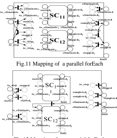
I. Mapping of forEach activity

(6)

Fig.11 Mapping of a parallel forEach

Fig.12 Mapping of a sequential forEach

IV. ANEXAMPLE

Based on mapping rules given above, an example is given in this section to show how a BPEL-based service composition is mapped onto a GSPN. The example is given in Fig.13. The sample is mapped into a GSPN shown in Fig.14. Primitive activities are represented by timed transitions while local computations and choice makings are represented by immediate transitions. Timed transitions td6-9 are used to express the transmission

delays of link signals. Note that, illustrations of activities and scopes look simpler and less detailed than figures given earlier in section.3 because unused transitions and places are omitted for brevity. Also note that, inhibition arcs from all transitions to the to_terminate place are also omitted.

V. STOCHASTIC MODELING

In this section, we will explain how to translate a GSPN mapped in section.4 into a stochastic state-transition system and derive its probabilistic state-transition matrix. For a GSPN mapped using rules given in section.3, let X(t) denote the set of timed transitions at time t (execution begins at time 0), then its state-space S can be obtained in a traversal way. The state space of the GSPN shown in Fig.14 is partially given in Table.I. As shown, state s3 is an absorbing state because it involves

execution of <exit> activity which leads to a sudden termination of the entire process.

TABLE I. STATE SPACE

state operational timed

transition state

operational timed transition

s1

(initial) {td1} s5 {td3}

s2 {td2, td3} s6 {td5} s3

(absorbing) {td2, td4} s7

{td6, td7, td8, td9}

s4 {td2} ……. ……

Fig.13 A sample service composition built on BPEL X(t) is a continuous-time homogeneous Markov chain with its infinitesimal generator matrix Q given by

,

, ,

1 | |,

(

)

(

)

0

l

m

td TISET

l m

ti TISET _i _j

i j i r

r S r i

td

pe ti

if s

s

q

if i

j

else

λ

∈

≤ ≤ ≠

⎧

∗

→

⎪

=

_⎨

−

=

⎪

⎩

∏

(7)

Where

λ

(

td

_l

)

denotes execution rate of transition

td

_l,

|

S

|

denotes the number of states in the state space and

,

i j

q

denotes the transition rate from state

s

_i to

s

_j.

Relation

,

l td TISET

i j

s

→

s

implies that

s

_j is the resulting

state of

s

_i if timed transition

td

_l and the set of immediate transitions TISET fire. Those resulting states are viewed as different types in the Markovian chain according to the phase-type property. The proof of Eq.2 is given below.

Fig.14 The GSPN derived from the BPEL sample

Proof

According to the Kolmogorov forward function, the

Q

matrix can be obtained as

j

i

j

i

t

p

t

p

q

ij t ij t ij

₌

≠

⎪

⎩

⎪⎪

⎨

⎧

∆

−

∆

=

→ ∆ → ∆

1 )

(

lim

)

(

lim

0 0 (3)

where

p

_ij

(

∆

t

)

denote the probability that the transition from state

s

i to

s

j is accomplished within a

infinitesimal period

∆

t

.

Let

STOP

_ij denote the set of timed transitions which

become inactive in the transition from

s

_i to

s

_j,

ACT

_i

denote and the set of timed transitions labeled by state

s

_i,

i

ED

denote the execution duration of timed transition

i

td

, respectively. We have

( )

( ) ( )

( )

( ) { } { }

( ) (1 )

m l ij o i ij

l o

m l ij o i ij

ij i j

m l o

ti TISET td STOP td ACT STOP

td t td t

m

ti TISET td STOP td ACT STOP

p t

pe ti P ED t P ED t

pe ti e λ e λ

≠

∈ ∈ ∈ −

− ∗∆ − ∗∆

∈ ∈ ∈ −

∆

= ∗ < ∆ ∗ ≥ ∆

= ∗ − ∗

∏

(4)

Consequently, we have

(( )) ( ) ( ) ( ) 0 ( ( )) 0 0 (1 )

( ( )) ( lim )

(1 )

( ( )) ( lim ) lim

( ( )

l o

l ij o i ij

m

tdl t

l ij o

m o i ij

td t td t

td STOP td ACT STOP

ij i j m

t ti TISET td STOP td t m t t

ti TISET td ACT STOP

m

e e

q pe ti

t

e pe ti e

t pe ti λ λ λ λ − ×∆ − ∗∆ − ∗∆ ∈ ∈ − ≠ _{∆ →} ∈ ∈ − ×∆ ∆ → ∆ → ∈ ∈ − − × = ∗ ∆ − = ∗ × ∆ =

∏

( ) 0 (1 ) ) lim l l ij m td t td STOP t ti TISET e t λ − ×∆ ∈ ∆ → ∈ − ∗ ∆

∏

(5) According to the equation above, we can conclude that

( )

0 _| _{| 1} _| _{| 0}

( ( )) ( ) _| _{| 1} _{{ }}

m

ij ij ij i j

l m

ij ij l ti TISET

if STOP or STOP q _td _{pe ti}

if STOP and STOP td

λ ≠

∈

⎧ _> ₌

⎪

= ⎨ _× ₌ ₌

⎪⎩

∏

(6) As for

q

_ij where

i

=

j

, we have

1 | |,

0 0

0

1 | |, 1 | |,

(

)

(

) 1

lim

(

)

lim

iw w S w i ii ii t t iw iw t

w S w i w S w i

(8)

VI. PERFORMANCEEVALUATION

The performance of a software system is mainly expressed as the number (the more the better) of tasks that system can accomplish in a given duration or the time (the shorter the better) that system takes to accomplish a given task. The latter is also known as completion time. Time is a common and universal measure of quality. The philosophy behind a time-based strategy usually demands that software systems deliver the most value as rapidly as possible. Shorter completion time allows for a faster production of service, thus providing efficiency and reducing cost. In this paper, we use expected-process-normal-completion-time (EPNCT for simple) as the metric of service performance. From the view of state transition, EPNCT denotes the expected duration for initial state to reach normal termination, ie. the absorbing state indicating normal completion of BPEL processes. A normal completion is achieved when execution of all activities and scopes are completed and no fault/compensation/termination/exit activities have occurred. Note that, according to [1] event handlers are considered a part of the normal behavior of the scope, unlike fault/compensation/termination handlers. Therefore, execution of event handlers is captured by the calculation of EPNCT.

To evaluate EPNCT, we first have to evaluate expected duration for each state to reach the absorbing state of normal termination (EDT(i)). We have:

i i

i

1 | |, , ( )

0 if s is the normal completion state

if s is an abnormal state

( ) if all immediate succeeding states of s have EDT of

( ) 1

+ ik else

k S k i EDT k

ii i

EDT i

q EDT k

q ≤ ≤ ≠ <∞ TEMP

⎧

⎪ _∞ ⎪⎪

= ∞⎨ ∞

⎪ _∗

⎪ −

⎪⎩

∑

(8)

where abnormal states are those which involve execution of fault/compensation/termination handlers or

<exit> activity (for instance state s3 in Table.I),

1

ii

q

−

is

the expected elapsing duration of state

s

_i and TEMPi is

an intermediate variable given by

1 | |, , ( )

i ik

k S k i EDT k

TEMP

q

≤ ≤ ≠ <∞

=

∑

(9) Eq.8 implies that the EDT of a certain state is simply its expected elapsing duration plus weighted EDT of its immediately succeeding states (excluding abnormal states and those which lead to abnormal states).

Based on observations above, we have that EPNCT is obtained as EDT of the initial state

(1)

EPNCT

=

EDT

(10) VII. EXPERIMENTSANDCONFIDENCEINTERVAL

ANALYSIS

In this section, we carry out an experimental study on the sample in Fig.14 and use experimental results to validate analytical methods introduced in earlier sections. In a real scenario, the parameters of the service components are described by Service Level Agreements.

As our aim is to present a methodology for evaluating performance, we used 3 groups of sample parameter settings given in Table.II. Please remember that these do not have realistic meanings, but have been chosen just to obtain experimental results.

Experiments are conducted on the sample given in Fig.14 and experimental performance results are obtained using a Monte-carlo procedure. Monte-carlo simulation is a flexible performance that it consists of a computer program that behaves like the system under study. The stochastic behaviors and events of target system are generated using pseudo-random number generators. The execution of a computer simulation is comparable to conducting an in-vitro experiment on the target system. Outputs of simulation procedure are treated as random observations (samples) of the system under study.

The Monte-carlo procedure conducts 10000 simulation runs of the sample. In each run, random generators are used to generate execution durations of executed primitive activities and link delays according to their execution rates. Random selectors following uniform distribution with range [0-1] are used to decide satisfaction of conditions C1-6 and decisions on

conditional branches are made according to those satisfaction results. When each simulation run terminates, process-completion-time is calculated and recorded based on execution durations of involved primitive activities if current simulation run results in a successful termination.

Fig.15 Histogram chart of process-normal-completion-time of the first parameter setting

Fig.16 Histogram chart of process-normal-completion-time of the second parameter setting

Fig.17 Histogram chart of process-normal-completion-time of the third parameter setting

(9)

process-normal-completion-time are illustrated in Fig.15-17. Those figures suggest process-normal-completion-time closely converge to normal distribution. Therefore, we use normal distribution as the fitting function to obtain 95% confidence intervals of EPNCT. On the other hand, analytical results of EPNCT are also obtained using methods introduced in earlier sections. Comparisons in Fig.18 indicate analytical estimates of EPNCT are perfectly covered by corresponding confidence intervals for all groups of parameter settings. The coverage indicates analytical methods introduced earlier are validated by experiments.

TABLE II. PARAMETER SETTINGS

Activities and links

Execution rates(1)

L1 0.23 0.43 0.25

L2 0.19 0.29 0.58

A1 0.45 0.18 0.68

A2 0.33 0.34 0.41

A3 0.5 0.66 0.22

A4 0.28 0.38 0.49

A5 0.48 0.49 0.78

A6 0.63 0.46 0.33

A7 0.75 0.25 0.30

A8 0.36 0.26 0.45

A9 0.53 0.74 0.62

A10 0.77 0.68 0.62

A11 0.27 0.87 0.52

A12 0.61 0.53 0.71

<exit> 0.35 0.46 0.64

<onMessage

m1> 0.56 0.33 0.29 Conditions _{probability (1)}Satisfaction _{probability (2)}Satisfaction _{probability (3)}Satisfaction

C1 0.5 0.25 0.65

C2 0.95 0.98 0.93

C3 0.05 0.02 0.07

C4 0.99 0.97 0.99

C5 0.96 0.94 0.96

C6 0.97 0.93 0.95

Fig.18 Analytical results vs. confidence intervals

VIII. CONCLUSIONS

This paper introduced a stochastic approach for integrating performance prediction into service composition processes described by BPEL. The proposed approach employs GSPN as the intermediate representation and bases itself on mapping rules which can translate primitive activities, structured activities, scopes and handlers into GSPN fragments. Based on a state-transition analysis and calculations on its corresponding Markov chain, analytical estimate of expected-process-normal-completion-time is obtained. To validate the approach, we also conduct Monte-carlo experiments based on different parameter settings and show theoretical results covered by corresponding 95% confidence intervals.

REFERENCES

[1] Alves, A., Arkin, A., Askary, S., Barreto, C., Bloch, B.,

Curbera, F., Ford, M., Goland, Y., Guizar, A., Kartha, N., Liu, C.K., Khalaf, R., Konig, D., Marin, M., Mehta, V., Thatte, S., Rijn, D.v.d., Yendluri, P., Yiu, A.: Web Services Business Process Execution Language Version 2.0. OASIS standard, Organization for the Advancement of Structured Information Standards (OASIS) (2007)

[2] Chun Ouyang, Eric Verbeek, Wil M. P. van der Aalst,

Stephan Breutel, Marlon Dumas, Arthur H. M. ter Hofstede: Formal semantics and analysis of control flow in WS-BPEL. Sci. Comput. Program. 67(2-3): 162-198 (2007)

[3] Chun Ouyang, Marlon Dumas, Arthur H. M. ter Hofstede,

Wil M. P. van der Aalst: From BPMN Process Models to BPEL Web Services. ICWS 2006: 285-292

[4] Niels Lohmann, Peter Massuthe, Christian Stahl, Daniela

Weinberg: Analyzing interacting WS-BPEL processes using flexible model generation. Data Knowl. Eng. 64(1): 38-54 (2008)

[5] Yanping Yang, QingPing Tan, Yong Xiao, Feng Liu,

Jinshan Yu: Transform BPEL Workflow into Hierarchical CP-Nets to Make Tool Support for Veri¯cation. APWeb 2006: 275-284

[6] Yanping Yang, QingPing Tan, Yong Xiao: Model

Transformation Based Verification of Web Services Composition. GCC 2005: 71-76

[7] Guofu Zhou, Chongyi Yuan: Mapping PUNITY to UniNet.

J. Comput. Sci. Technol. 18(3): 378-387 (2003).

[8] Enric Pastor, Oriol Roig, Jordi Cortadella, Rosa M. Badia:

Petri Net Analysis Using Boolean Manipulation Application and Theory of Petri Nets 1994: 416-435

[9] Moser, S., Martens, A., Gorlach, K., Amme, W., Godlinski,