Detection of LSB Matching Steganography using the Envelope of Histogram

Detection of LSB Matching Steganography using

the Envelope of Histogram

Jun Zhang

School of Information Science

Guangdong University of Business Studies ,Guangzhou ,P.R. China Email: [email protected]

Yuping Hu and Zhibin Yuan Department of Software Enginerring

Guangdong University of Business Studies ,Guangzhou ,P.R. China Email: [email protected]

Abstract—As well-known, it is hard to detect LSB matching steganography when cover images are scans of photographs, which usually have high-frequency noise. This paper proposes a novel steganalysis method for this issue by making use of the following two facts: One is the local maxima of an image histogram decrease and the local minima increase after LSB matching steganography. As a result, the area between upper envelope and lower envelope of the histogram of a stego image will be smaller than that of a cover image. The other is LSB matching embedding in the spatial domain of an image corresponds to low-pass filtering of the histogram. So, there are some differences in the high order statistical moments of high frequencies of the histogram. Based on these facts, this paper constructs a novel feature vector to distinguish between stego and cover images. Experimental results show the proposed scheme has better performance than some state-of-the-art steganalyzers in the literature.

Index Terms—Steganalysis, LSB matching, Image

I. INTRODUCTION

Steganography has received considerable interest during the last few years, especially after anecdotal reports alleged that this technology was used by terrorist. Steganography seeks to provide a covert communication channel between two parties. It is commonly framed as the prisoners’ problem [1-2]: Two prisoners, Alice and Bob, are permitted to communicate between one another, while under the surveillance of a Warden. The Warden, Eve, is free to examine all transmitted contents between Alice and Bob and must decide whether such transmissions include a covert message. If there is a covert message, then the communication between the prisoners will be prevented. The content that doesn’t contain the covert message is referred to as the cover content, which might be an image, video, audio or text. Otherwise it is referred to as the stego content. The goal of Alice and Bob is to develop steganographic algorithms so that a covert message is undetectable by Eve. Nowadays, a wide variety of steganographic algorithms have been proposed.

They can be categorized in two groups: Spatial domain techniques like least significant bit (LSB) replacement, LSB matching [3], Pixel Value Differencing [4] and Stochastic Modulation [5]; Transform domain techniques like Outguess [6], F5 [7], Patchwork [8].

In the other side, steganalysis attempts to defeat the goal of steganography. It aims to expose the presence of the hidden message, equivalently, to discriminate the stego content from the cover content. Steganalysis are commonly categorized as either targeted or blind. Targeted steganalysis seeks to detect the use of a known steganographic algorithm. It can reveal the covert message or even estimate the embedding ratio with the knowledge of the steganographic algorithm [9-14]. Blind steganalysis seeks to detect a range of steganographic algorithms, possibly including previously unknown algorithms. Blind steganalysis first extract some features from contents, or more specifically, images, then select or design a classifier, and train the classifier using the features extracted from training image sets, and lastly, classify the features for an identifying given images [15-22]. Usually, it is likely that steganalysis methods that target a specific embedding scheme can give more accurate and reliable results than blind steganalysis ones. However, blind approaches are more practical because of their flexibility and ability to be quickly adjusted to new or completely unknown steganographic methods.

by one. However, it will never be decremented. The converse is true for odd-valued pixels. Rather than simple replace the LSB with the desired message bit, LSB matching scheme randomly increments or decrements the corresponding pixel value when the desired message bit is different from the LSB. Due to remove the asymmetry of odd and even pixels, detection of LSB matching is known to be much more difficult than detecting LSB replacement.

There are some detectors for LSB matching steganography in the literature. Unfortunately, their performances are often low when cover images have high-frequency noise, such as high resolution scans of photographs. This paper addresses this issue. Section II first reviews three state-of-the-art steganalyzers used to detect LSB matching steganography, which are algorithms of Harmsen et al. [23],Ker [24] and Goljan et al.[25]. They can be roughly considered as sharing a common architecture, namely (i) feature extraction in some domain and (ii) Fisher Linear Discriminant (FLD) analysis to obtain a 2-class classifier.

Section III examines the effect of LSB matching steganography on the intensity histogram. We show that the local maxima of the histogram of images will decrease and the local minima will increase after LSB matching embedding. This property can be used to define a feature to detect LSB matching steganography. The feature is the area between upper envelope and lower envelope of the histogram. Moreover, since LSB matching embedding in the spatial domain of an image corresponds to low-pass filtering of the histogram, there must be some differences in the high order statistical moments of high frequencies of the histogram. According to these facts, we construct a novel feature vector to distinguish between stego and cover images.

Section IV explains the details of the proposed steganalyzer. In section V, we give experimental results and compare the performance with the three state-of-the-art steganalyzers. The paper is concluded in Section VI.

II. RELATED WORK

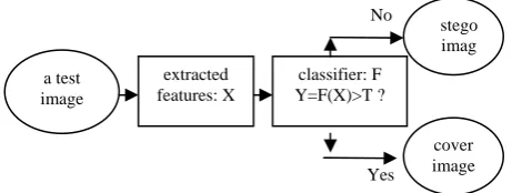
Steganalysis can be modeled as a classify problem as shown in Fig.1.

Input a test image, extract some features X form it, then a classify function F is used to identify it. If F(X) is more than a threshold T then the test image belongs to cover class otherwise it belongs to stego class. The performance of steganalysis depends on two factors: one is which features of images are selected. The other is which classify functions are used. The latter is well studied in the fields of pattern recognize and machine learning, which usually

Figure 1. The common architecture of steganalyzer

is Fisher Linear Discriminant(FLD), Support Vector Machine (SVM) or Neural Network (NN). The former is the key issue in steganalysis. That means: a steganalyzer must find out some features of images that are sensitive to embedding modifications so that it can distinguish between cover and stego images. In this section, we will briefly review the three state-of-the-art steganalyzers for LSB matching steganography and focus on how to select features in these methods.

A. Center of Mass of the Histogram Characteristic Function

One of the first steganalyzers was proposed by Harmsen and Pearlman [23]. They model LSB matching steganography as independent additive noise. Due to the fact that noise adding in the spatial domain corresponds to low-pass filtering of the histogram, the histogram of stego images has less power in high frequencies than the histogram of cover images. So, the center of mass of the Histogram Characteristic Function

H

, which is obtained by Fourier transform of the histogram , will decrease after LSB matching embedding. Then, it was used as a feature for distinguishing between cover and stego images. This scheme is called a Histogram Characteristic Function steganalysis (HCF). The center of mass of HCF is calculated as follows:

h

( )

( )

( )

∑

∑

= =

∗

=

₁₂₇

0 127

0

i i

i

H

i

H

i

H

C

(1)

This technique has quite good performance for detecting LSB matching steganography in RGB color images. However, it performs very poorly in grayscale images indeed.

B. Center of mass of the Adjacency Histogram Characteristic Function

Ker suggested that HCF scheme has bad performance in grayscale images since it is a lack of sparsity in the histogram [24]. He then proposed to use a two-dimensional adjacency histogram, expressing how often each pixel intensity is observed horizontally next to each other. Because adjacent pixels tend to have close intensities, this histogram is sparse off the diagonal. He showed that LSB matching steganography also reduces to low-pass filtering the adjacency histogram and defined a center of mass of the adjacency histogram characteristic function as follows:

a test image

extracted features: X

classifier: F Y=F(X)>T ?

stego imag

cover image Yes

No

( )

(

)

( )

( )

∑

∑

= =

∗

+

=

₁₂₇

0 127

0

,

,

i i

j

i

H

j

i

H

j

i

H

In addition, to reduce the variability of this feature across images, Ker recommended computing the same center of mass using a downsampled version of the image. For discussing next, the former is referred to as AD-HCF and the latter is referred to as CAD-HCF.

C. Wavelet Absolute Moment

Holotyak and Fridrich [18] described a blind steganalysis approach based on classifying higher-order statistical features derived from an estimation of the stego signal in the wavelet domain. Goljan [25] presented an improved version of Holotyak’s method by using absolute moments of the noise residual. The proposed approach is flexible and enable reliable detection of presence of secret messages embedded using a wide range of steganographic methods that include LSB matching, LSB replacement, Stochastic Modulation, and others. This steganalyzer is referred to as WAM. The algorithm of WAM is described as follows:

Step 1: Input a test image I

Step 2:

I

is transformed by discrete wavelet transforms (DWT). The results include 4 subimages, which are denoted as

LL

,

LH

,

HL

,

HH

Step 3: The three high frequency subimages are denoised by wavelet filter, and the results are denoted as

respectively. '

' '

,

,

HL

HH

LH

Step 4: Compute the residual subimages:

' '

'

,

,

HL

HL

HH

HH

LH

LH

HL HH

LH

=

−

Δ

=

−

Δ

=

−

Δ

Step 5: Calculate high-order absolute moments of the residual subimages:

(

)

i LH LH

−

mean

Δ

Δ

,

Δ

_HL

−

mean

(

Δ

_HL

)

i ,

(

)

i HH HH

−

mean

Δ

Δ

, i=1…9.

Finally, they use all these 27 data as a feature vector to distinguish between cover and stego images.

WAM steganalysis performs very well for cover images that were previously compressed using JPEG, but its accuracy is very low in cover images scanned from photographs.

III. ANALYSIS FOR LSBMATCHING STEGANOGRAPHY

A. LSB matching steganography

We assume that images are grayscale ones, which means their pixels will be in the range 0…255. The pixels at location of cover image and stego image are

denoted as and , respectively. In LSB

matching steganography, one message bit is embedded at pixel by applying the following formula (3).

)

,

(

i

j

)

,

(

i

j

p

c

p

s

(

i

,

j

)

)

,

(

i

j

p

_c

Where

r

is an i.i.d. random variable with uniform distribution on

{

−1,+1

}

,

b

is the message bit, and

( )

p

LSB is the least significant bit of

p

. The pixels of a cover image are selected (pseudo) randomly using a shared stego key for embedding. Rather than simply replacing the LSB with the desired message bit (LSB replacement scheme), the corresponding pixel value is randomly incremented or decremented in LSB matching steganography. However, if pixels are 0 and 255, we force them to be 1 and 244, respectively. So, without the asymmetry of LSB replacement, it is much more difficult to detect the LSB matching steganography than LSB replacement.

( )

(

( )

)

( )

(

( )

)

( )

(

( )

)

⎪ ⎩ ⎪ ⎨ ⎧

< ≠

−

=

> ≠

+ =

0 & ,

1 ,

,

,

0 & ,

1 ,

) , (

r j i p LSB b if j

i p

j i p LSB b if j

i p

r j i p LSB b if j

i p

j i p

c c

c c

c c

s

(3)

B. Effects of LSB Matching steganography on Histogram

The histogram of the cover image is calculated by using following formula:

( ) ( ) ( )

n

{

i

j

p

i

j

n

}

h

_c

=

,

_c

,

=

(4) Where is grayscale level in the range 0…255. The histogram stands for the number of pixels with grayscale level .

n

n

Assume that a maximal-length hidden message (1 bit per pixel of the cover image) is embedded and message bit is also an i.i.d. random variable with uniform distribution on

b

{ }

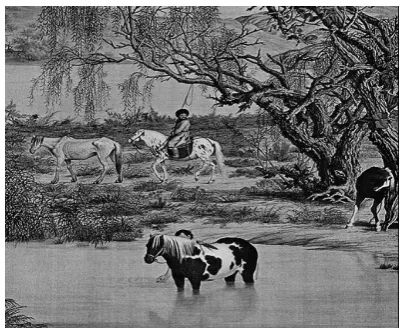
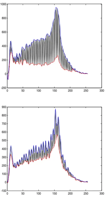
0,1 . We now discuss the effects on histogram of the cover image by LSB matching steganography.

Let us begin with an example of LSB matching steganography. Fig.2 shows a cover image, which is the photography of artwork with size 512*512. Fig.3 shows the histogram of the cover image and stego image in which 512*512 message bits are embedded by LSB matching method. As we can see the histogram of the stego image is more smooth than that of the cover image.

Moreover, the local maximums become smaller and the local minimums become larger. This is true by following theoretical analysis indeed.

Definition 1. In a histogram function , is a local maximum point if the two inequalities

( )

h

*

n

( ) (

n* ≥hn* −1

)

h and h

( ) (

n* ≥hn*+1

)

are true and one of inequalities is strict.

Definition 2. In a histogram function , is a local minimum point if the two inequalities

( )

h

n

*

( ) (

_n* ≤_hn*−1

)

h and _h

( ) (

_n* ≤_hn*+1

)

are true and one of inequalities is strict.

Lemma 1. If s a local maximum point of histogram

then *

n

i

( ) ( )

* *

n

h

n

h

_s

<

_c . Here, the h_c

( )

and h_s

( )

stand for histograms of the cover and stego image, respectively.

0 50 100 150 200 250 300 -200 0 200 400 600 800 1000

0 50 100 150 200 250 300 -100 0 100 200 300 400 500 600 700 800 900

Figure 3. The top one is the histogram of the cover image shown in Fig.2 and the bootom is that of the stego image

Proof. We assume

r

, message bit

b

and

( )

(

p i j

)

LSB c , in formula (3) are random variables with

uniform distribution independently. Then, a pixel p_s

( )

i,j of the stego image is obtained by following probability:

(

)

(

(

(

( )

)

) (

)

)

( )

(

)

(

) (

4 / 1 2 / 1 2 / 1 1 , 1 , 1 = ⋅ = = ⋅ ≠ =

)

= ∧ ≠ = + = r P j i p LSB b P r j i p LSB b P p p P c c c s

Similarly, P

(

p_s = p_c −1

)

=1/4 and P

(

p_s= p_c

)

=1/2. Denote the number of pixels that their grayscale level are from

n

up ton+1, and down to after LSB embedding as

n

n−1

(

→ +1

)

Δ n n and Δ

(

n→n−1

)

,

respectively. Then,

(

n→n+1

) ( ) (

=h n ⋅P p_s= p_c+1

) ( )

=hn /4

Δ .

Similarly, Δ

(

n→n−1

) ( )

=h n /4. So,

( ) ( ) (

) (

)

(

) (

)

( ) ( )

( )

( )

(

)

( )

(

(

( ) ( )

) ( ) (

(

)

)

( )

/4 1 1 /4 1 /4 1 /4 /4 1 1 1 1 * * * * * * * c * * * * * * * * * * * * * * n h n h n h n h n h n h n h n h n h n h n h n n n n n n n n n h n h c c c c c c c c c c c s < + − + − − − = + + − + − − = → + Δ + → − Δ + − → Δ − + → Δ − =

)

Symmetrically, we can deduce the following lemma 2.

Lemma 2. If s a local minimum point of histogram then *

n

i

( ) ( )

* *

n

h

n

h

_s

>

_c .

The lemmas show the fact that after LSB matching the local maxima of an image histogram decrease and the local minima increase. So, we can expect the area between the upper envelope and lower envelope of the histogram of the cover image will be larger than that of the histogram of the stego image. As a result, we use it as one of features to distinguish between cover and stego images. The area can be calculated by the following procedure: Identify all the local extrema, then connect them by a cubic spline line to form the upper envelope

u

( )

. Repeat the procedure for the local minima to produce the lower envelope

l

( )

, as shown in Fig.3. The area is defined as the absolute of the difference between the upper envelope and lower envelope.That is,

_∑

_{( ) ( )}

= − =255 0 n n l n u

S (5) Fig.3 clearly shows the area of the histogram of the cover image is larger than that of the stego image. Their areas are 59765 and 41288, respectively.

0 10 20 30 40 50 60 70 80 90 100 1

2 3 4 5 6 7 8 9x 10

4

Figure 4. The aeras of envelope of histogram of cover and stego images. The symbols ‘*’ and ‘o’ stand for

c of cover images and of

stego images, respectively.

S Ss

images like Fig.2. The results are shown in Fig.4, in which the symbols ‘*’ and ‘o’ stand for of cover images and

of stego images, respectively. As we can see, are

almost lager than . So we can use the area of envelope of histogram as a discriminator to separate cover images from stego images.

c

S

s

S

S

c

s

S

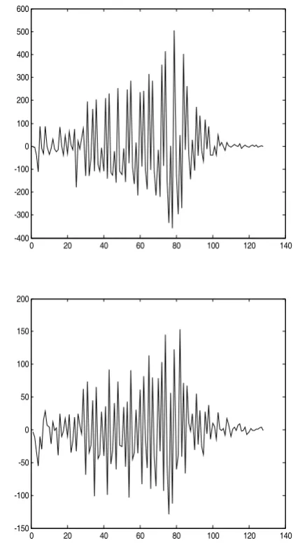
Finally, we investigate another feature for steganlaysis. LSB matching scheme can be modeled as independent additive noise, it leads to low pass filtering on the intensity histogram. As a result, the histogram of the stego image has less power in high frequencies than the histogram of the cover image [23]. We gain the high frequencies of the histogram by discrete wavelet transform shown in Fig.5. The top one is the high frequency coefficients of the histogram of the cover image and the bottom is that of the stego image. As we can see, there are some differences in the high order statistical moments of high frequencies of the histograms. For example, the standard deviations of the top and bottom one are 143.45, 50.55, respectively. That means the standard deviation of histogram of the stego image is smaller than that of the cover image. This is almost true for each image according to our experiments. So, we can use the standard deviation as another feature to distinguish between stego and cover images. Combined with the feature mentioned above, we can expect to improve accuracy of detection.

IV. STEGANALYSIS ALGORITHM

As discussed above, we present two features for steganalysis. Moreover, we introduce another feature based on the local extremum of histogram in our previous work [26]. Making use of these three features, we propose the following steganalysis algorithm.

Step 1. Given a test image, calculate the histogram of the image by formula (4).

Step 2. Compute all local maximums and minimums of

0 20 40 60 80 100 120 140 -400

-300 -200 -100 0 100 200 300 400 500 600

0 20 40 60 80 100 120 140 -150

-100 -50 0 50 100 150 200

Figure 5. The top one is the high frequency coefficients of histogram of the cover image and the bootom is that of the stego image

the histogram.

Step 3. Work out the area between the upper envelope and lower envelope of the histogram by formula (5), denoted as

f

₁.

Step 4. Transform the histogram by DWT, and then calculate the high order statistical moments of the high frequencies. In our experiments we just select the standard deviation, denoted as

f

2.

Step 5. Calculate the sum of absolute differences between each local extremum and its neighbors in the histogram. That is,

*

n

( ) (

) ( ) (

)

(

)

∑

− − + − +

=

*

1

1 * *

* * 3

n

n h n h n

h n h f

(6)

Step 6. Combine , and to form the three- dimensional feature vector. Then, the Fisher linear

1

discriminator (FLD) is introduced to classify cover and stego images. The FLD is a simple classification method which finds an optimal linear projection of the features. Advantages of the FLD method include reasonably fast training, very fast use, and no training parameters to select. In the FLD, the feature space is projected on a one-dimensional space, where various decision rules can be applied for determining the classification thresholds.

Finally, we use receiver operating characteristic curves (ROC) to evaluate the performance of our method and compare it with other methods. ROC can show how the false positives and true positives vary as the detection threshold is adjusted [27].

V. EXPERIMENTAL RESULTS

It is an established fact nowadays that detection of LSB matching steganography is significantly more difficult for never compressed images, grayscale images, and scans of photographs, and notably easier for images that were previously processed using JPEG or for color images. So our tests will focus on the following dataset, which includes never compressed scaned images.

The dataset is derived from the Corel Image Database, which includes 2000 color images scanned from photographs of artworks. The original images are 24-bit, 512*768 pixels, never compressed and they usually have high level of noise. In our experiments, we crop the original color images into 512*512 pixels and covert them to grayscales. Here, cropping was preferred over resizing, in order to avoid introducing artifacts due to resampling with interpolation.

For this dataset, the following procedure was performed for the steganalyzer to calculate its ROC [28]:

1) Apply LSB embedding steganography with embedding rate p to all images in the dataset D to

obtain the dateset of stego images *

D ;

2) Separate both dataset into a training set

( ) ( )

{

D I ,D* I

}

and a test set

{

D( )I′ ,D*( )I′

}

, where I is a subset of the image indexes and '

I is its complement. The size of the training set was set to be equal to 50% of the dataset size;

3) For the steganalyzer under test, compute the associated feature vector for all images in the training set and perform FLD analysis to obtained the trained projection vector

v

;

4) For the steganalyzer under test, compute the associated feature vector for all images in the test set, and project the feature vector onto

v

;

5) Compare the resulting scalar values to a threshold

τ

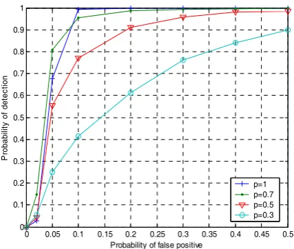
and record the probabilities of false positives and true positives for different values of the threshold in order to obtain the Receiver Operating Characteristic curve of the steganalyzer.

Firstly, we evaluate the performance of our method under embedding rate p = 0.3, p = 0.5, p = 0.7and

0 0.05 0.1 0.15 0.2 0.25 0.3 0.35 0.4 0.45 0.5 0

0.1 0.2 0.3 0.4 0.5 0.6 0.7 0.8 0.9 1

Probability of false positive

P

roba

bi

lit

y o

f det

ec

tio

n

p=1 p=0.7 p=0.5 p=0.3

Figure 6. ROCs for the proposed method with various embedding rate

0 0.05 0.1 0.15 0.2 0.25 0.3 0.35 0.4 0.45 0.5 0

0.1 0.2 0.3 0.4 0.5 0.6 0.7 0.8 0.9 1

Probability of false positive

P

rob

ab

ilit

y of

det

ec

tio

n

HCF AD-HCF CAD-HCF WAM Our method

Figure 7. ROCs for the five steganalyzers under embedding rate 0.5.

1

=

p . The experimental results are shown in Fig.6. As we can see, when the embedding rate increases the performance will improve. For example, at false positive rate 50% the detection rates are 90%, 98%, 100% and 100% for the embedding rates 0.3, 0.5, 0.7 and 1.

Then, fixing the embedding rate we compare our method with the Histogram Characteristic Function steganalysis (HCF) [23], the adjacency HCF-COM version (AD-HCF) and the calibrated adjacency HCF-COM version (CAD-HCF) of Ker’s method [24], and Goljan’s method (WAM) [25].

5 . 0

= p

WAM method to distinguish between the stego signal and noise naturally present in images. (3) The performance of AD-HCF is almost the same as that of HCF in this dataset.

(4) The calibrated detector (CAD-HCF) performs worse than the standard detector ( AD-HCF). That means the calibration technique fails when a hidden message only 50% of the maximum is embedded.

VI. CONCLUSION

The detection of LSB matching steganography remains unresolved, especially for the uncompressed grayscale images with high level of noise, such as scans of photographs. In this paper, we present a novel steganalysis scheme for this issue. By analyzing the embedding algorithm of LSB matching steganography, we prove the fact that the local maximum of histogram of a cover image decrease and local minimum increase after message bits are embedded. Moreover, due to the fact that the histogram of the stego image has less power in high frequencies than that of the histogram of the cover image, there are some differences in the high order statistical moments of high frequencies. Based on these facts, we construct a new feature vector and use the FLD to distinguish between the cover and stego images. The experimental results show the proposed scheme is superior to the HCF and WAM methods in the dataset of scans of photographs.

It is well-known that the performance of current state-of-the-art steganalyzers for detection of LSB matching steganography is highly sensitive to the datasets from different sources. No detectors have yet proven universally reliable. Further work is needed to understand this variability and to characterize it for particular algorithms, and also to develop a hybrid method that combines all advantages of the related methods.

ACKNOWLEDGMENT

This work was supported by National Natural Science Foundation of China under Grant No.60873198, Guangdong Natural Science Foundation (N0:06023961) and Natural Science Foundation of Department of Education of Guangdong Province (N0:05Z013)

REFERENCES

[1] G. J. Simmons, “The prisoners’ problem and the subliminal channel,” in Advances in Cryptology: Proceedings of CRYPTO’83. Plenum Pub Corp, pp. 51–67, 1984

[2] I. J. Cox, Ton Kalker, Georg Pakura and Machia Scheel, “Information transmission and steganography, ” Lecture Notes in Computer Science, vol. 3710, pp.15-29, 2005

[3] Q. Liu, A. Sung, J. Xu, and B. Ribeiro, “Image complexity and feature extraction for steganalysis of LSB,” in ICPR06, pp. II:267–270, 2006

[4] N. Wu and M. Hwang, “Data hiding: current status and key issues,” International Journal of Network Security, vol. 4, no. 1, pp. 1–9, 2007

[5] J. Fidich and M. Goljan, “Digital image steganography using stochastic modulation,” SPIE Electronic Imaging, pp. 191–202, 2003

[6] N. Provos, “Defending against statistical steganalysis,” Usenix Security Symp., pp. 323–335, 2001

[7] A. Westfeld, “F5 - a steganographic algorithm,,” Springer-Verlag Berlin Hd, pp. 289–302, 2001

[8] R. Anderson and F. Peticolas, “On the limits of steganography,” IEEE Journal of Selected Areas in Comunication, pp. 474–481, 1998

[9] J. Fridrich, M. Goljan, R. Du, “Reliable detection of LSB steganography in color and grayscale images, in: Proceedings of ACM Workshop Multimedia Security, pp. 27–30, 2001

[10] S. Dumitrescu, X. Wu, Z. Wang, “Detection of LSB steganography via sample pair analysis,” IEEE Trans. Signal Process, 51 (7), pp.1995–2007, 2003

[11] T. Zhang, X.J. Ping, “A new approach to reliable detection of LSB steganography in natural image,” Signal Process. 83 (10), pp.545–548 ,2003

[12] J. Fridrich, “Feature-based steganalysis for JPEG images and its implications for future design of steganographic schemes,” in: Proceedings of sixth Information Hiding Workshop, Lecture Notes in Computer Science, vol. 3200, pp. 67–81, 2004

[13] J. Fridrich, M. Goljan, D. Hogea, “Steganalysis of JPEG images: breaking the F5 algorithm,” in: Proceedings of fifth International Workshop on Information Hiding, Lecture Notes in Computer Science, vol. 2578, Springer, Berlin, pp. 310–323, 2002.

[14] Andrew D. Ker, “Quantitive evaluation of pairs and RS

steganalysis.,” Proc.SPIE Security, Steganography,Watermarking Multimedia Contents, vol.5306, E. J. Delp III and P. W. Wong, Eds., pp. 83-97, 2004

[15] I. Avcibas, N. Memon, B. Sankur, “Steganalysis of watermarking techniques using image quality metrics,” in: Proceedings of the SPIE, Security and Watermarking of Multimedia Contents II, vol. 4314, pp. 523–531, 2000

[16] H. Farid, “Detecting hidden messages using higher-order statistical models,” in: Proceedings of IEEE International Conference on Image processing, vol. 2, pp. 905–908, 2002

[17] S. Lyu, H. Farid, “Steganalysis using color wavelet statistics and oneclass support vector machines,” in: Proceedings of the SPIE, Security, Steganography, and Watermarking of Multimedia Contents VI, vol. 5306, pp. 35–45, 2004

[18] T. Holotyak, J. Fridrich, S. Voloshynovskiy:, “Blind Statistical Steganalysis of Additive Steganography Using Wavelet Higher Order Statistics,” The 9th IFIP 6 TC-11 Conference on Communications and Multimedia Security. Lecture Notes in Computer Science, vol. 3677, pp.273-274,2005

[19] J. Fridrich, David Soukal, Miroslav Goljan, “Maximum likelihood estimation of length of secret message embedded using steganography in spatial domain,” Proc.SPIE,5681,pp.595-606,2005

[20] Y.Q. Shi, G.R. Xuan, C.Y. Yang et al. , “Effective steganalysis based on statistical moments of wavelet characteristic function,” in: Proceedings of IEEE International Conference on Information Technology: Coding and Computing, pp. 68–773, 2005

Lecture Notes in Computer Science, vol. 3727, Springer, Berlin, pp. 62–277, 2005

[22] Y. Wang, P. Moulin, “Optimized feature extraction for learning-based image steganalysis, ” IEEE Trans. Inf. Forensics Secur. 2 (1) ,pp. 31–45,2007

[23] J. Harmsen, W. Pearlman, “Higher-order statistical steganalysis of palette images,” Proc. SPIE Security Watermarking Multimedia Contents, vol. 5020, E. J. Delp III and P.W.Wong, Eds., pp. 131-142, 2003

[24] Andrew D. Ker, “Steganalysis of LSB Matching in Grayscale Images,” IEEE Signal Processing Letters, Vol. 12, No. 6, pp.441-444, 2005

[25] M. Goljan, J. Fridrich, and T. Holotyak, “New blind steganalysis and its implications,” in Security, Steganography, and Watermarking of Multimedia Contents VIII, ser. Proceedings of SPIE, vol. 6072, pp.1–13, 2006

[26] Jun Zhang, I. J. Cox, G. Doerr, “Steganalysis for LSB matching in images with high-frequency noise,” Proc. IEEE Workshop on Multimedia Signal Processing, pp. 385-388, 2007

[27] R. O. Duda, P. E. Hart, and D. G. Stork, Pattern Classification, 2nd ed. Wiley-Interscience, 2001

[28] G. Cancelli, G. Doerr , M. Barni, and I. J. Cox, “A comparative study of ±1 steganalyzers,” Proc. IEEE International Workshop on Multimedia Signal Processing, pp.791-796, 2008

Jun Zhangwas born in Sichuan, China in 1966. He received his Ph.D degree in computer science from Huazhong Universityof Science & Technology, China in 2003 and his M.Sc. degree in Mathematics from Lanzhou University in 1993.

He had been a visiting postdoctoral Researcher in University College London, UK under Prof. Ingemar Cox’s supervision. Now, he is the rector of Information Science School, Guangdong University of Business Studies. His research interest is information security such as data hiding, watermarking and privacy protection. In this field, He has published more than 30 papers. Moreover he had been in charge of some projects sponsored by National Natural Science Foundation of China and Guangdong Natural Science Foundation. He served as many workshop chairs, advisory committee or program committee member of various international IEEE.

Yuping Hu was born in 1969. He received his B.S. degree in celestial survey from Chinese Academy of Science, China, in 1996 and his Ph.D. degree in computer science from Huazhong University of Science and Technology, Wuhan , China in 2005. He is currently pursuing the postdoctoral research in computer applications from Central South University, Changsha, China.

Dr.Hu is a professor in the School of Information science, Guangdong University of Business Studies, Guangzhou, China. His current research interests include digital watermarking, image processing, multimedia and network security.