Community structure based on circular flow in a large-scale transaction network

(1)

R E S E A R C H

Open Access

Community structure based on circular

flow in a large-scale transaction network

Yuichi Kichikawa

1*

, Hiroshi Iyetomi

1,3

, Takashi Iino

1

and Hiroyasu Inoue

2

*Correspondence:

[email protected]

1_{Faculty of Science, Niigata} University, Niigata, 950-2181, Japan Full list of author information is available at the end of the article

Abstract

The objective of this study is to shed new light on the industrial flow structure embedded in microscopic supplier-buyer relations. We first construct directed networks from actual data from interfirm transaction relations in Japan; as one

example, the dataset compiled by the Tokyo Shoko Research, Ltd. in 2016 contains five million links between one million firms. Then, we analyze the industrial flow structure of such a large-scale network with a special emphasis on its hierarchy and circularity. The Helmholtz-Hodge decomposition enables us to break down the flow on a directed network into two flow components: gradient flow and circular flow. The gradient flow between a pair of nodes is given by the difference of their potentials obtained by the Helmholtz-Hodge decomposition. The gradient flow runs from a node with higher potential to a node with lower potential; hence, the potential of a node shows its hierarchical position in a network. On the other hand, the circular flow component illuminates feedback loops built in a network. The potential values averaged over firms classified by the major industrial category describe hierarchical characteristics of sectors. The ordering of sectors according to the potential agrees well with the general idea of the supply chain. We also identify industrially integrated clusters of firms by applying a flow-based community detection method to the extracted circular flow network. We then find that each of the major communities is characterized by its main industry, forming a hierarchical supply chain with feedback loops by complementary industries such as transport and services.

Keywords: Production network, Helmholtz-Hodge decomposition, Visualization

Introduction

In general, interactions between individuals are considered to play an important role in the economy. For instance, firms are connected to each other directly or indirectly through their business transactions. A firm buys materials from suppliers and sells its products to customers. These transactions are so essential to firms that one cannot iso-late the dynamics of individual firms from the entire economic system. Firms’ production activities thus give rise to a complex network; also, examining economic phenomena from the perspective of networks can provide a variety of new insights into economic phenomena.

Conventionally, the industrial structure and economic ripple effects have been studied on the basis of the input-output tables (Leontief1986). Furthermore, a network-theoretic point of view was incorporated into the input-output analysis to elucidate complex interindustrial flow structures within or across the sectors (Slater1977; 1978; Carvalho

(2)

2008; McNerney et al.2013; Contreras and Fagiolo2014). However, such classification of firms by industry may be too formal for a reliable macroscopic picture of the economy.

Recently, firm-level network analyses based on a comprehensive database of interfirm transaction relations have begun to appear (Atalay et al. 2011; Acemoglu et al.2012; Cainelli et al.2012; Luo et al.2012; Watanabe et al.2015; Letizia and Lillo2018; Goto et al.2017). Economists as well as physicists have recognized the importance of taking an explicit account of interfirm links in order to understand economic issues, such as the origin of business cycles and the possibility of a chain reaction in firm bankruptcies.

Very recently, we have studied (Chakraborty et al.2018) the structure of a Japanese pro-duction network with one million firms and five million supplier-customer links. We first constructed a directed production network from the actual data of interfirm transaction relations and found that they form a tightly knit structure with a giant strongly connected component surrounded by two half-shells constituting incoming-flow and outgoing-flow components for the core. The hierarchical structure of communities was then elucidated by a flow-based multilevel community detection method (Rosvall and Bergstrom2011), and most of the irreducible communities were found to be on the second level. The com-position of some of the major communities, including overexpressions of industrial and regional components, as well as hierarchical connections between the communities, was studied in detail.

The hierarchy of the production network is expected to emerge from self-organization of the supply chain in the industrial system. This is the general view on evolutionary processes in complex systems (Holland2000; Anderson1972). Here, we emphasize that we should also pay attention to the inner loops of production, giving rise to a nonlinear feedback mechanism in the system, because they can be engines for economic growth. The priority production system adopted by the Japanese government just after World War II is an illustrative application of this idea (Vestal1995). It was intended to stimulate recovery of the nation’s economy so damaged by concentrating public investment into coal mining and steel production. Production of steel needs electricity generated from coal, and mining of coal needs machinery made of steel. Such an industrial loop formed by the three industries, mining, steel production, and machinery manufacturing, led to autonomous growth of the economy.

The objective of this study is to advance the previous empirical analysis (Chakraborty et al.2018) on the industrial flow structure embedded in microscopic supplier-buyer rela-tions with a special emphasis on its circularity. To delve further into the flow structure of the transaction network with firms as nodes, we take advantage of a mathematical tool called the Helmholtz-Hodge decomposition (Jiang et al.2011; Bhatia et al.2013). It allows us to decompose the flow on a directed network into a gradient flow component and a circular flow component.

(3)

elucidate circular flow structure in the production network. The final section summarizes the results obtained here.

Interfirm transaction data

The present analysis is based on the big data of 4,974,802 transaction relations between 1,066,037 firms in Japan that was collected by the Tokyo Shoko Research, Ltd. (TSR) in 2016.1These data virtually cover the entire amount of industrial activities in Japan. We regard firms as nodes and transaction relations between them as directed links spanning from suppliers to customers to construct the latest production network in Japan. Since information on the volume of each transaction is not available, we assume that all the links have the same weight.

In addition to the information on transactions between firms, various attributes of indi-vidual firms are available. For simplicity of analyses, we use two attributes of each firm, namely, industrial sector and geographical location of the head office. Firms are cate-gorized into 20 sectors and 47 prefectures. Readers are referred to the previous paper (Chakraborty et al.2018) for more detailed information on the dataset.2

Helmholtz-Hodge decomposition

In general, one can write flowFijrunning from nodeito nodejin a directed network as follows:

Fij=Fij(p)+Fij(c), (1)

where we assume that the magnitude ofFijon the network is given by the following:

|Fij| =

⎧ ⎪ ⎨ ⎪ ⎩

1 (singly connected in one way) 0 (doubly connected in both ways) 0 (not connected)

(2)

Since information on the volume of transactions is not available in the TSR dataset, we adopt such a simplified flow structure. The first termF_ij(p)on the right-hand side of Eq. (1) denotes the gradient flow from nodeito nodejwhich is given by the following:

F_ij(p)=wij

φi−φj

, (3)

where φi is the Helmholtz-Hodge potential associated with node i and wij is a posi-tive weight for linkage between nodesiandj. We assume that the weightwijtakes the following values depending on how the two nodes are connected:

wij=

⎧ ⎪ ⎨ ⎪ ⎩

1 (singly connected in one way) 2 (doubly connected in both ways) 0 (not connected)

(4)

The Helmholtz-Hodge potential of nodes in a directed network identifies their hierarchi-cal positions in its flow structure. In the network built with only gradient flow, nodes are perfectly ranked; the gradient flow always runs from a node with higher potential to a node with lower potential. On the other hand, the second termF_ij(c)denotes the circular

1_{This is the largest connected component in the network obtained from the original data, containing}_99.3%_{of all active}

firms listed in the data.

2_{In this study, sector I (Wholesale & retail trade) in (Chakraborty et al.}₂₀₁₈_{) was separated into two sectors, Wholesale}

(4)

flow component in which incoming flow and outgoing flow are exactly balanced at each node:

j

F_ij(c)=0 , (5)

so that there is no hierarchy among nodes in the circular flow network. The circular flow component illuminates feedback loops embedded in the system.

Additionally, one can determine the potentialφi for every node by minimizing the squared difference between the actual flow and the gradient flow:

I= 1 2

i<j

w−_ij1 Fij−Fij(p)

2

, (6)

where the double summation excludes pairs of nodes that are not connected. This is a variational formulation of the Helmholtz-Hodge decomposition. Subtracting the gradient flow thus determined from the original flow leaves the loop flow. In addition, to remove arbitrariness in the potential determination, we impose the following condition onφi:

i

φi=0 . (7)

To quantify to what extent the flow of a directed network has hierarchical and circu-lar characteristics, we introduce two measures for the gradient flow and circucircu-lar flow components associated with each nodeias follows:

ξ(p)

i = 1 2 jw −1

ij F(

p)

ij

2

j<kw

−1

jk

F_jk2

, (8)

ξ(c)

i = 1 2 jw −1 ij F

(c)

ij

2

j<kw

−1

jk

Fjk

2. (9)

Summation ofξ_i(p)andξ_i(c)over all nodes yields generalized formulas for the gradient and loop ratios (Fujiki and Haruna2014; Haruna and Fujiki2016), respectively:

γ =

i

ξ(p)

i , (10)

λ =

i

ξ(c)

i . (11)

Because of the orthogonality between the gradient flow and the circular flow vectors, the sum of the two ratios amounts to unity:

γ +λ=1 (12)

If a network is completely hierarchical (circular),γ = 1(0)andλ=0(1). One can thus use either of the two ratios to characterize the overall flow structure of a directed network. This can be considered as ranking the nodes according to the hierarchical structure of the network.

(5)

accomplishes this by minimizing the penalty function called agony, and De Bacco et al. (2018) by minimizing the energy of the physical model. Determining φ to minimize Eq. (6) corresponds to the Helmholtz-Hodge decomposition. The expression of energy minimization of the physical model is one of the variants of the Helmholtz-Hodge decom-position. Generally, the method of optimizing the penalty function is computationally expensive, but the computational cost of the Helmholtz-Hodge decomposition and phys-ical model is not so cumbersome because it only needs to solve a set of linear equations. The major difference between Helmholtz-Hodge decomposition and other methods is the Helmholtz-Hodge decomposition allows us to treat hierarchies and cycles on equal foot-ing. The Helmholtz-Hodge decomposition has a strong advantage of providing a unified representation of the flow structure of a directed network not only in terms of hierarchy but also in terms of circularity. In this paper, we focus on circularity as well as hierarchy, taking advantage of the Helmholtz-Hodge decomposition.

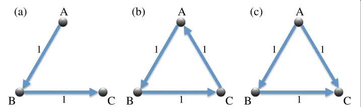
Finally, we illustrate the Helmholtz-Hodge decomposition with examples of triangular transaction networks in Fig.1. The first example shown in Fig.1a is a completely hierar-chical network withφA =1,φB = 0, andφC = −1, while the second one in Fig.1b is a completely circular network. The third example in Fig.1c is a mixed network with both hierarchical and circular characteristics. Its gradient flow component, Fig.2a, is deter-mined byφA = 2/3,φB =0, andφC= −2/3. The circular flow component is a loop of flow with magnitude 1/3, as shown in Fig.2b.

Bow-tie decomposition

To elucidate flow structure in the TSR transaction network, we begin with the bow-tie decomposition of the network, which has been widely used to understand the flow struc-ture of various complex networks including the worldwide web and metabolic networks. The decomposition classifies nodes in a directed network according to the way in which they are mutually connected: IN component, GSCC (giant strongly connected compo-nent), OUT component, and others. The GSCC is the largest group of nodes in which any pairs of nodes are connected bidirectionally by two directed paths. The IN component is a collection of nodes that have a path to the GSCC, but no reverse path to come back from the GSCC. The OUT component is defined in the other way around, that is, a collection of nodes that are reachable only from the GSCC. From their definition, these classifica-tions of nodes provide an overall view on the hierarchical structure of the network. In the previous paper (Chakraborty et al.2018), however, we named such a structure of the TSR network the “walnut” structure instead of the bow-tie structure after its shape. Because

A

B

C

A

B

C

A

B

C

(a)

(b)

(c)

1

1 1 1

1

(6)

A

B

C

A

B

C

(b)

(a)

1/3

2/3

4/3

Fig. 2Gradient flow component (a) and circular flow component (b) of the triangular network as shown in Fig.1c, according to the Helmholtz-Hodge decomposition

the IN and OUT components are not as separated as the two wings of a bow-tie, they are more similar to two halves of a walnut shell, surrounding the central GSCC core.

Table1lists the numbers of firms belonging to the IN, GSCC, OUT and other com-ponents of the TSR network. The results are compared with the corresponding numbers of firms averaged over 1000 random networks with the same degree distribution as that of the original network. We observe no significant difference in the bow-tie parameters between the original and randomized networks. However, Table1also shows that com-plete randomization of the network destroys the bow-tie structure; virtually all nodes constitute the GSCC.

In contrast, the distributions of the Helmholtz-Hodge potential shown by the histogram in Fig.3exhibit a significant difference between the two deep networks; the flow structure of the network is influenced by the randomization process.

The potential distributions of IN, GSCC, and OUT in the original network are well-overlapped compared with the randomized network with the same degree sequence. In particular, the distributions of IN and OUT of the randomized network are quite separated, but the corresponding distributions of the original network are substantially overlapped. For a quantitative argument, we define the following overlap integral of two distribution functions:

J=

f(x)·g(x)dx

f2₍_x₎_dx_g2₍_x₎_dx

. (13)

The overlap integralJtakes a value within the range of 0 ≤ J ≤ 1;Jtakes the unity for f(x)∝g(x). In the TSR network, the overlap integral of the potential distributions for the

Table 1The numbers of firms belonging to the IN, GSCC, OUT and other components of the TSR transaction network

TSR Random TSR Completely Random

IN 219,927 212, 415(181.9) 10, 395(105.1)

GSCC 530,174 560, 876₍212.5₎ 1, 045, 150₍154.6₎

OUT 278,880 263, 412(201.7) 10, 388(108.1)

Others 37,056 25, 701(162.5) 9(3.0)

Total 1,066,037 1, 062, 404₍82.4₎ 1, 065, 942₍10.1₎

(7)

Fig. 3Distributions of the Helmholtz-Hodge potential for firms in the IN component (red), GSCC (green), and OUT component (blue) of the TSR transaction network. The left and right panels show the results for the original network and one sample of the randomized networks with the same degree sequence, respectively

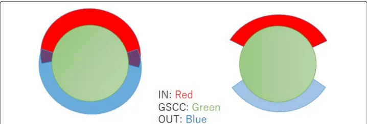
IN and OUT components isJ(TSR)=0.125. On the other hand, randmized networks with the same degree sequence take much smaller values ofJ, for instance,J_0.01(rand) = 0.00021 andJ_0.05(rand)=0.00020, whereJ_0.01(rand)andJ_0.05(rand)are the 1% and 5% significance level ofJfor 1,000 samples, respectively. These numerical results establish the conceptual difference between the bow-tie structure and the walnut structure, as shown in Fig.4, in a statisti-cally meaningful way. We emphasize that the structure is not essentially determined by the degree distribution, but by more detailed properties on the linkage of the network.

Figure5shows the distribution of firms in such bow-tie components of the TSR net-work across sectors. The sectors such as Construction, Information & Communications, and Scientific Research, Professional & Technical Services are important constituents in the IN component. Mining, Manufacturing, Transport & Postal, and Wholesale sectors are key players in the GSCC. The important sectors in the OUT component include Retail Trade, Finance & Insurance, Accommodations, Eating/Drinking Services, Living-related/Personal & Amusement Services, and Education, Learning Support. We thus see that each component of the bow-tie structure in the production network has its own industrial characteristics. The main industries in the GSCC form an integrated core of economic activities in Japan.

Results and discussion

We first obtained an optimized layout of the network in three-dimensional space by incor-porating information of the Helmholtz-Hodge potential for individual nodes. The result is displayed in Fig.6. Nodes are aligned in thezdirection according to their values of the

(8)

Fig. 5Distribution of firms in the IN (red), GSCC (green), OUT (blue) and other components (gray) of the TSR transaction network across sectors

Helmholtz-Hodge potential; basically, transaction flows are from top to bottom. On the other hand, thexandycoordinates of nodes are determined by minimizing the poten-tial energy in a spring-electric model in which nodes with direct transaction relations are connected to each other by a spring and all nodes have an identical electric charge to maintain distance from disconnected nodes. In Fig.6, nodes belonging to the differ-ent walnut compondiffer-ents are distinguished with differdiffer-ent colors. Figure7shows half-cut cross-sections of the 3D images of the network, as shown in Fig.6. The walnut structure is also clearly visible in this visualization. The GSCC is certainly sandwiched between the IN component on the upstream side and the OUT component on the downstream side. However, the potential values in the three components are distributed so widely that even the potential distributions of the peripheral components are not well separated. These

Z

Y X

Z

Z Y

Y X

X

(9)

X Y

Z

Z Y

Y X

X

Fig. 7Half-cut cross-sections of the 3D images of the TSR network as shown in Fig.6

results agree with our naming convention of the flow structure of the transaction network as a walnut structure.

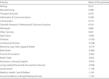
Figure8resolves the three potential distributions in Fig.3into those within individual sectors. The averaged value of the potential for firms in each sector is given in Table2. The results, listed in their descending order, describe hierarchical characteristics of the sectors in the transaction network. For instance, the manufacturing sector is located at the upstream side compared with the wholesale and retail trade sectors. The hierarchical ordering of sectors is in harmony with the general idea of the supply chain. However, the potential values are widely distributed from upstream to downstream even within the same sectors, except for Finance & Insurance, Medical, Health Care & Welfare, and Government. This fact indicates that major sectors such as Manufacturing, Construction, Wholesale and Retail trades have appreciable hierarchical structure in and of themselves. We turn own attention to the gradient ratioγ and loop ratioλfor the whole network and the GSCC of the transaction network.3_{The results are shown in Table}₃ _together

with the corresponding results for the two kinds of random networks in parallel with Table1. The hierarchy is significantly developed in the original network compared with the randomized networks. This is understandable because hierarchical structure is in general a manifestation of self-organization in complex systems (Holland2000; Anderson 1972); it is a formation of supply chains in the economic system. Although randomizing the network with a preserved degree distribution does not change the walnut structure considerably, the randomization procedure has an appreciable influence on the balance between the hierarchy and circularity of the network. We have similar results for the GSCC of the original network. The hierarchy is slightly stronger than the circularity even in the GSCC consisting only of nodes that are mutually connected in both ways. In con-trast, the circularity dominates the flow structure of the corresponding network that has been completely randomized.

The hierarchical flow is dominant in the IN component, which has mainly one-way flow to the GSCC because of its definition. This is also true for the OUT component. On the other hand, the GSCC has a more complicated flow structure; both hierarchical and circular flow components coexist in it. This is because any pairs of nodes in the GSCC are connected bidirectionally by at least two directed paths. We thus expect that firms in the GSCC constitute the core of the production activities, while firms in the IN and OUT parts, forming a thin layer for the GSCC, are just peripherals.

(10)

Fig. 8Resolution of the three potential distributions in the left panel of Fig.3into those within sectors

For the purpose of this study, therefore, we hereafter concentrate on the flow struc-ture of the GSCC, especially its circularity. To identify important loops in the cir-cular flow network on the GSCC, we adopt the map equation method (Rosvall and Bergstrom2008; 2011) for community detection. It is an information-theoretic method based on an idea that random walkers should stay in looping communities for a long

Table 2The averaged values of the Helmholtz-Hodge potential for firms in individual sectors, which are listed in their descending order corresponding to the direction of upstream to downstream in the TSR transaction network

Industry Mean of the potential

Mining 0.412

Manufacturing 0.388

Transport & Postal 0.353

Information & Communications 0.348

Construction 0.216

Scientific Research, Professional & Technical Services 0.103

Wholesale 0.084

Other Services 0.041

Agriculture -0.081

Fisheries -0.100

Compound Services -0.188

Electricity, Gas, Heat Supply & Water -0.274

Real Estate -0.380

Finance & Insurance -0.562

Retail Trade -0.602

Education, Learning Support -0.910

Living-related/Personal & Amusement Services -0.998

Government -1.100

Medical, Health Care & Welfare -1.247

Accommodations, Eating/Drinking Services -1.253

(11)

Table 3Gradient ratioγand loop ratioλfor the whole network and the GSCC of the TSR transaction network

γ λ

Whole network

TSR 0.648 0.352

Random TSR 0.537₍0.0001₎ 0.463₍0.0001₎

Completely Random 0.214(0.0003) 0.786(0.0003)

GSCC

TSR 0.537 0.463

Random TSR 0.386(0.0001) 0.614(0.0001)

Completely Random 0.200(0.0002) 0.800(0.0002)

The results are compared with the corresponding ratios averaged over 1000 random networks with the same degree distribution and 1000 completely random networks with the same number of links as that of the original network; the figures in parentheses show the standard deviation associated with each of the average values

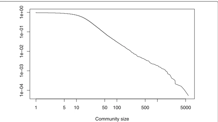
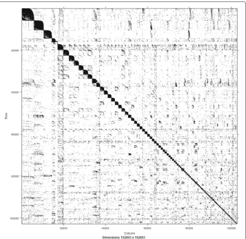
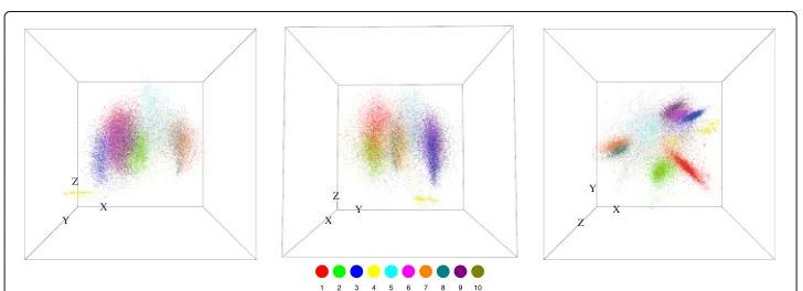
time. Figure 9 demonstrates that the communities so detected have a size distribu-tion of the long-tail form. The total number of communities is 18,660, and the largest community has approximately 5000 firms. Figure 10 depicts the adjacency matrix of the circular flow network in which nodes are ordered according to the community assignment. It shows the community detection works well because links are sparse between the communities and are considerably dense within the communities. The 10 largest communities are illuminated in Fig.11with the same node configuration as in Figs.6and7.

Figure12shows the histogram of the Helmholtz-Hodge potential differenceφof links for the 1st-6th communities, whereφ = φi−φj is the potential difference between nodes i and j at both ends of linksFij(> 0). A positive value of φ indicates a link directed from the upstream side to the downstream side, while a negative value ofφ, a link in the reversed direction. The distribution ofφis significantly shifted to the posi-tive side except for the 5th community. It means that the main flow from the upstream to

1 5 10 50 100 500 5000

1e−04

1e−03

1e−02

1e−01

1e+00

Community size

(12)

Fig. 10 The adjacency matrix of the circular flow network sorted in descending order regarding the community size, where it shows the top 100 largest communities

the downstream dominates over the feedback flow in those communities. On the other hand, the 5th community shows the distribution ofφthat is quite symmetrical around

φ=0. This indicates that the exceptional community has well-developed circular flow structure, which will be addressed later.

(13)

Fig. 11 The 10 largest communities in the circular flow network on the GSCC of the transaction network, visualized in three-dimensional space with three different points of view. The same configuration of firms is used as in Fig.6.

X Y Z

Z Y Z

X

Y X

1 2 3 4 5 6 7 8 9 10

(14)

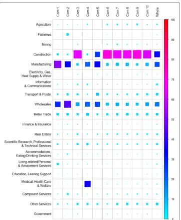
Fig. 13 Industrial characterization of the 10 largest communities obtained for the circular flow network on the GSCC by share of sectors to which their constituent firms belong. The size of each square is proportional to share of the corresponding industry in the specified community. Additionally, its share value (in percentage) is represented by the color coding

(15)

(16)

Table 4Number of firms for each industry type that belongs to the 6 largest communities

Industry type #firms

Community 1

Manufacture of textile mill products 2547

Wholesale trade (textile and apparel) 1222

Miscellaneous living-related and personal services 226

Retail trade (dry goods, apparel and apparel accessories) 184

Miscellaneous wholesale trade 171

Wholesale trade (building materials, minerals and metals, etc.) 93

Professional services 81

Miscellaneous of manufacturing industries 78

Construction work, general work including public and private construction work 74

Miscellaneous business services 73

Community 2

Wholesale trade (food and beverages) 1850

Manufacture of food 1383

Retail trade (food and beverage) 151

Fisheries 150

Cooperative association 124

Road freight transport 99

Aquaculture 60

Miscellaneous retail trade 57

Warehousing 41

Community 3

Construction work by specialist contractor, except equipment installation work 802

Equipment installation work 672

Wholesale trade (machinery and equipment) 165

Technical services 82

Machinery and equipment 72

Industry types are according to the middle classification of the TSR industry type classification

the medical and health services are general hospitals and clinics. Community 5 contains many firms in the manufacture and wholesale of metal products and construction. On the other hand, most of the firms in communities 3 and 6 are those in the construction industry. Although the industrial distributions of the construction communities resemble each other closely, they are clearly distinguished by their regional characteristics. In fact, communities 3 and 6 are dominated by firms in Okinawa and Kagoshima, respectively. We note that Okinawa is considerably isolated from the mainland in the whole industry.

(17)

Table 5Continuation of Table4

Industry type #firms

Community 4

Medical and other health services 956

Manufacture of chemical and allied products 349

Wholesale trade (food and beverages) 69

Miscellaneous business services 55

Manufacture of food 49

Professional services 42

Community 5

Manufacture of fabricated metal products 305

Manufacture of iron and steel 212

Manufacture of production machinery 120

Manufacture of general-purpose machinery 79

Community 6

Manufacture of ceramic, stone and clay products 62

Agriculture 31

Technical services 31

(18)

Table 6Table of the number of firmsncfor each industry type in the community, and the number of

firmsn_cthat has the top 10% of theξ(c)/ξ(p)value within the community

Industry type n_c nc nc/nc

Community 1

Manufacture of textile mill products 144 2547 0.057

Wholesale trade (textile and apparel) 71 1222 0.058

Miscellaneous wholesale trade 37 171 0.216

Miscellaneous retail trade 21 58 0.362

Equipment installation work 19 59 0.322

Wholesale trade (building materials, minerals and metals, etc.) 19 93 0.204

Construction work by specialist contractor, except equipment installation work 18 71 0.254

Miscellaneous of manufacturing industries 18 78 0.231

Road freight transport 17 59 0.288

Wholesale trade (machinery and equipment) 17 71 0.239

Community 2

Wholesale trade (food and beverages) 154 1850 0.083

Manufacture of food 89 1383 0.064

Retail trade (food and beverage) 20 151 0.132

Fisheries 12 150 0.08

Cooperative association 12 124 0.097

Aquaculture 8 60 0.133

Construction work, general work including public and private construction work 7 40 0.175

Community 3

Machinery and equipment 18 72 0.25

Manufacture of ceramic, stone and clay products 10 65 0.154

Information services 10 29 0.345

The top-10 industry types ofncare listed in decreasing order

(19)

Table 7Continuation of Table6

Industry type n_c nc nc/nc

Community 4

Manufacture of chemical and allied products 18 349 0.052

Wholesale trade (food and beverages) 13 69 0.188

Miscellaneous business services 13 55 0.236

Professional services 10 42 0.238

Advertising 10 28 0.357

Technical services 10 23 0.435

Agriculture 9 25 0.36

Community 5

Manufacture of fabricated metal products 33 305 0.108

Manufacture of production machinery 18 120 0.15

Manufacture of general-purpose machinery 9 79 0.114

Miscellaneous business services 8 25 0.32

Community 6

Construction work, general work including public and private construction work 44 993 0.044 Construction work by specialist contractor, except equipment installation work 35 529 0.066

Manufacture of fabricated metal products 11 28 0.393

Manufacture of lumber and wood products 6 26 0.231

the manufacture and wholesale of pharmaceutical products exhibits high hierarchy, but technical services and advertising indicate high circularity. In community 5, construction work and wholesale trade (building materials, minerals and metals, etc.) show high hier-archy, while miscellaneous wholesale trade, equipment installation work and road freight transport largely contribute to the circularity. In fact, the miscellaneous wholesale trade particularly includes iron and steel primary product wholesale, steel crude product whole-sale and iron scrap wholewhole-sale trade, indicating that recycling steps of iron and steel are incorporated into the steel industry. This is why the flow structure of community 5 is so highly circular, as has been demonstrated.

(20)

hidden by its strong hierarchy. To overcome the difficulty, we exclusively examined the circular flow component and then applied the community detection to the network thus constructed. Each of the communities that we have detected consist of a hierarchical sup-ply chain of the main industry and feedback loops formed by firms in industries that complement the main industry. Specifically, we found that the transport industry plays an important role in forming the feedback structure for many of the major communities in the production network. In the previous study (Chakraborty et al.2018), on the other hand, the original flow network was decomposed into communities. Consequently, we were unsuccessful in detecting such industrially integrated clusters of firms as have been reported here.

Conclusions

The comprehensive dataset of interfirm transaction relations in Japan enabled us to study the industrial flow structure of the nation’s production network with a sound micro-scopic foundation. Particularly, we emphasized its hierarchy and circularity. The network was first decomposed into the walnut components according to their flow properties: IN, GSCC, OUT, and others. The flow structure of the walnut components except the GSCC is mainly hierarchical. By adopting the Helmholtz-Hodge decomposition, we sep-arated the flow structure of the GSCC of the network into two components: gradient flow and circular flow. The gradient flow between a pair of firms is given by the dif-ference of their potentials, and hence, the potential of a firm identifies its hierarchical position in the transaction network. On the other hand, the circular flow component illu-minates feedback loops built in the network. The potential values averaged over firms classified by the major industrial category describe hierarchical characteristics of sectors. The order of sectors determined by the potential calculation agrees well with the general idea of the supply chain. We also identified dominant clusters of firms forming feed-back loops by applying the map equation method to the extracted circular flow network. We found that both hierarchical and loop structures coexist within the major sectors, such as construction, manufacturing, and wholesales. We measured the magnitude of the contribution to the circular structure from each firm in the major communities. The measurement indicates that the main industry that characterizes the community exhibits high hierarchy and low circularity. On the other hand, most of the firms that contribute to the circular flow structure belong to industries complementary to the main industry, such as the transportation industry. These results suggest limitations of the conventional industrial classification scheme in analyzing economic activities, which may be replaced by a new classification scheme for firms based on the actual interfirm transactions.

Appendix A: Identification of nodes significantly contributing to the feedback structure.

(21)

(22)

flows passing through them and one reversed flow forming the feedback structure. This network can be decomposed into the gradient flow and the circular flow components by the Helmholtz-Hodge decomposition, as illustrated in Fig.15. For this gradient flow com-ponent, the potential differenceφbetween the adjacent layers takes the constant value of(n−1)/(n+1)throughout the intermediate layers, and the potential difference between the most upstream and the most downstream is thereby(m+1)φ. All of the gradient flows are thus directed from top to bottom with flux ofφ. In the circular flow compo-nent, each of thenparallel flows is also directed downward with flux ofc = 2/(n+1). These parallel flows join at the bottom node and go back to the top node to form a feed-back loop with flux ofnc= 2n/(n+1). On the feedback path, the direction of the loop flow is the same as that of the original flow, while that of the gradient flow is reversed from the original direction (Fij andFij(c)have the same sign, whileF

(p)

ij has the opposite sign). Quantitatively, the circular flow component plays a relatively important role for a node on the feedback path compared with that for a node on the main stream lines. This is as guaranteed by the following calculations.

Thus, the relative magnitude of ξ_i(c) in reference to ξ_i(p) for every node i is a good measure to identify the nodes that are important in the feedback structure.

For a nodeion the feedback path,ξ_i(p)andξ_i(c)are calculated as follows:

ξ(p)

i =

|φ|2

i<j|Fij|2 ∝

n−1 n+1

2

, (14)

ξ(c)

i =

(nc)2

i<j|Fij|2 ∝ 4n2

(n+1)2, (15)

hence:

ξ(c)

i

ξ(p)

i

= 4n2

(n−1)2. (16)

For a nodejon the main stream lines,ξ_j(c)/ξ_j(p)is likewise given by the following:

ξ(c) j

ξ(p) j

= 4

(n−1)2. (17)

Ifn1, then Eq. (16) takes a much larger value than Eq. (17).

Abbreviations

GSCC: Giant Strongly Connected Component; TSR: Tokyo Shoko Research

Acknowledgments

This study has been conducted as a part of the project “Large-scale Simulation and Analysis of Economic Network for Macro Prudential Policy” undertaken at the Research Institute of Economy, Trade and Industry (RIETI). This research used computational resources of the K computer provided by the RIKEN Center for Computational Science through the HPCI System Research project (Project ID: hp170242, hp180177).

Authors’ contributions

The paper was written collaboratively. The coauthors read and approved the final manuscript.

Funding

This research was also supported by MEXT as Exploratory Challenges on Post-K computer (Studies of Multilevel Spatiotemporal Simulation of Socioeconomic Phenomena) and JSPS KAKENHI Grant Numbers JP15KT0052, JP17KT0034, and JP18K03451.

Availability of data and materials

(23)

Competing interests

The authors declare that they have no competing interests.

Author details

1_{Faculty of Science, Niigata University, Niigata, 950-2181, Japan.}2_{Graduate School of Simulation Studies, University of}

Hyogo, Kobe, 650-0047, Japan.3_{The Canon Institute for Global Studies, Tokyo, 100-6511, Japan.}

Received: 1 March 2019 Accepted: 30 August 2019

References

Acemoglu D, Carvalho VM, Ozdaglar A, Tahbaz-Salehi A (2012) The network origins of aggregate fluctuations. Econometrica 80(5):1977–2016

Anderson PW (1972) More is different. Science 177(4047):393–396

Atalay E, Hortacsu A, Roberts J, Syverson C (2011) Network structure of production. Proc Natl Acad Sci 108(13):5199–5202 Bhatia H, Norgard G, Pascucci V, Bremer P-T (2013) The Helmholtz-Hodge decomposition—a survey. IEEE Trans Vis

Comput Graph 19(8):1386–1404

Cainelli G, Montresor S, Vittucci Marzetti G (2012) Production and financial linkages in inter-firm networks: structural variety, risk-sharing and resilience. J Evol Econ 22(4):711–734

Carvalho VM (2008) Aggregate Fluctuations and the Network Structure of Intersectoral Trade. The University of Chicago, Chicago

Chakraborty A, Kichikawa Y, Iino T, Iyetomi H, Inoue H, Fujiwara Y, Aoyama H (2018) Hierarchical communities in the walnut structure of the japanese production network. PloS ONE 13(8):0202739

Contreras MGA, Fagiolo G (2014) Propagation of economic shocks in input-output networks: A cross-country analysis. Phys Rev E 90(6):062812

De Bacco C, Larremore DB, Moore C (2018) A physical model for efficient ranking in networks. Sci Adv 4(7):8260 Fujiki Y, Haruna T (2014) Hodge decomposition of information flow on complex networks. In: Proceedings of the 8th

International Conference on Bioinspired Information and Communications Technologies. ICST (Institute for Computer Sciences, Social-Informatics and Telecommunications Engineering), Gent. pp 103–112

Goto H, Takayasu H, Takayasu M (2017) Estimating risk propagation between interacting firms on inter-firm complex network. PloS ONE 12(10):0185712

Haruna T, Fujiki Y (2016) Hodge decomposition of information flow on small-world networks. Frontiers Neural Circ 10:77 Holland JH (2000) Emergence: From Chaos to Order. OUP Oxford, Oxford

Jiang X, Lim L-H, Yao Y, Ye Y (2011) Statistical ranking and combinatorial Hodge theory. Math Program 127(1):203–244 Johnson S, Domínguez-García V, Donetti L, Muñoz MA (2014) Trophic coherence determines food-web stability. Proc Natl

Acad Sci 111(50):17923–17928

Letizia E, Lillo F (2018) Corporate payments networks and credit risk rating. Available at SSRN 3075019 Leontief W (1986) Input-output Economics. Oxford University Press, Oxford

Letizia E, Barucca P, Lillo F (2018) Resolution of ranking hierarchies in directed networks. PloS ONE 13(2):0191604 Luo J, Baldwin CY, Whitney DE, Magee CL (2012) The architecture of transaction networks: a comparative analysis of

hierarchy in two sectors. Ind Corp Chang 21(6):1307–1335

McNerney J, Fath BD, Silverberg G (2013) Network structure of inter-industry flows. Phys A Stat Mech Appl 392(24):6427–6441

Rosvall M, Bergstrom CT (2008) Maps of random walks on complex networks reveal community structure. Proc Natl Acad Sci 105(4):1118–1123

Rosvall, M, Bergstrom CT (2011) Multilevel compression of random walks on networks reveals hierarchical organization in large integrated systems. PloS ONE 6(4):18209

Slater P (1977) The determination of groups of functionally integrated industries in the united states using a 1967 interindustry flow table. Empir Econ 2(1):1–9

Slater, P (1978) The network structure of the united states input-output table. Empir Econ 3(1):49–70

Tatti N (2015) Hierarchies in directed networks. In: 2015 IEEE International Conference on Data Mining. IEEE, New York. pp 991–996

Vestal JE (1995) Planning for Change: Industrial Policy and Japanese Economic Development 1945-1990. Clarendon Press, Oxford

Watanabe T, Uesugi I, Ono A (2015) The Economics of Interfirm Networks, vol. 4. Springer, New York

Publisher’s Note