R E S E A R C H
Open Access
Solving the maximum subsequence sum
and related problems using BSP/CGM model
and multi-GPU CUDA
Anderson C. Lima
1†*, Rodrigo G. Branco
1†, Samuel Ferraz
1, Edson N. Cáceres
1, Roussian A. Gaioso
2†,
Wellington S. Martins
2and Siang W. Song
3Abstract
Background: The maximum subsequence problem finds a contiguous subsequence of the largest sum of a sequence ofnnumbers. Solutions to this problem are used in various branches of science, especially in applications of computational biology. The best sequential solution to the problem has an O(n)running time and uses dynamic programming. Although effective, this solution returns little information and disregards the existence of more than a maximum subsequence sum. Particularly in DNA analysis, if we find all maximum subsequence sums, we will also find all the possible pathogenicity islands, which are stretches with high possibility of causing some diseases.
Methods: We present new Bulk Synchronous Parallel/Coarse-Grained Multicomputer (BSP/CGM) parallel algorithms, which consider the existence of more than one subsequence of maximum sum, and are able to find solutions to three problems: the longest maximum subsequence sum, the shortest maximum subsequence sum, and the number of disjoint subsequences of maximum sum. To the best of our knowledge, there are no parallel BSP/CGM algorithms for the related problems. Taking advantage of the advent of general purpose graphics processing unit (GPGPU), we implemented our algorithms on multi-GPU with Compute Unified Device Architecture (CUDA) and, for comparison purposes, MPI and OpenMP implementations have also been developed.
Results: The algorithms presented good speedups, as confirmed by experimental results. They usepprocessors and require O(n/p)parallel time with a constant number of communication rounds for the algorithm of the maximum subsequence sum and O(logp)communication rounds, with O(n/p)local computation per round, for the algorithms of the related problems.
Conclusions: We concluded that our algorithms for the maximum subsequence sum and related problems are unique and effective. We also believe that the BSP/CGM model can guide parallel implementations in modern architectures such as GPGPU/CUDA. As future work, we intend to extend these results to arrays with higher dimensions and compute all maximal subsequences in a given interval.
Keywords: Parallel algorithms, Multicore, GPGPU, BSP/CGM, Maximum subsequence sum problem
*Correspondence: [email protected] A short version of this paper was presented at the ICCS-2015 [8] †Equal Contribution
1Faculdade de Computação da Universidade Federal de Mato Grosso do Sul, Cidade Universitária, C.P: 549 Campo Grande, MS, Brasil
Full list of author information is available at the end of the article
Background
Given a sequence ofn numbers, the task of finding the
contiguous subsequence, with maximum sum over all subsequences of the given sequence, is called the max-imum subsequence sum problem [2]. We also refer to this problem as the 1D maximum subsequence sum prob-lem. The solution of this problem arises in many areas of science, such as computational biology, where many appli-cations require the solution of the maximum subsequence sum problem. Among these, finding regions of DNA that
are rich or poor in nucleotides G and C (CG-content).
The GC-content is especially important in the search for pathogenicity islands [9]. Another biological applica-tion is the identificaapplica-tion of transmembrane domains in protein sequences. This is an important application and represents one of the important tasks to understand the structure of a protein or the membrane topology [12].
The best sequential algorithm for the maximum
sub-sequence sum problem, has O(n) time complexity [2].
Despite being a simple and fast algorithm, it yields lit-tle information about the maximum subsequence sum. The output returns only the value of the maximum subse-quence sum. The algorithm does not consider the length (number of elements) and existence of more than one maximum subsequence sum. The pseudocode is illus-trated in Algorithm 1.
Algorithm 1 Maximum subsequence sum (MSqS)
(sequential)
Require: SequenceSof integers.
Ensure: The value of the maximum subsequence sum ofS.
1: MaxSoFar←0.
2: MaxEndingHere←0.
3: fori=1 tondo
4: MaxEndingHere←max(MaxEndingHere+S[i], 0).
5: MaxSoFar←max(MaxSoFar, MaxEndingHere).
6: end for
Previous works have reported good parallel solutions for the maximum subsequence sum problem. Qiu and Akl presented algorithms for the 1D (subsequence) and 2D (subarray) versions of the problem [11]. Their algorithms work on interconnection networks (hypercube and star) of lengthp, using O(n/p+logp)parallel time withp pro-cessors in version 1D [11]. Zhaofang Wen presented a parallel random access machine (PRAM) algorithm using O(logn) parallel time with O(n/logn) processors [16]. Perumalla and Deo also presented a PRAM algorithm with the same time complexity and number of processors [10]. A Bulk Synchronous Parallel/Coarse-Grained Mul-ticomputer (BSP/CGM) algorithm for this problem was presented by Alves et al. using O(n/p)parallel time with
p processors and a constant number of communication
rounds [1].
In this paper, we revisit the maximum subsequence sum problem and propose solutions to three related problems: the longest maximum subsequence sum, the shortest maximum subsequence sum, and the number of disjoint subsequences of maximum sum.
As far as we know, there are no parallel BSP/CGM algorithms for these three problems. The basis of our solution involves several variations of prefix sum in parallel [7].
The algorithms use p processors and require O(n/p)
parallel time with a constant number of communication rounds for the algorithm of the maximum subsequence sum and O(logp) communication rounds, with O(n/p)
local computation per round, for the algorithms of the related problems.
In order to show the efficiency not only in theory but also in practice, the algorithms were implemented on a machine with multiple GPUs using compute unified device architecture (CUDA). We also implemented the algorithms with MPI and OpenMP.
This paper is organized as follows. The “Methods” section defines the basic and related problems, dis-cusses the extension of a solution already known, and presents our proposed BSP/CGM algorithms. The imple-mentations and results are presented in the “Results” section.
Finally, the “Conclusions” section presents the conclu-sions and future work.
Methods The problems
The basic problem of the 1D maximum subsequence sum may be defined formally as follows. For simplicity we con-sider the numbers to be integers. Concon-sider a sequence
Xn = (x1,x2,. . .,xn)ofnintegers. A subsequence is any
contiguous segment (xi,. . .,xj) of Xn, where 1 ≤ i ≤
j ≤ n. The 1D maximum subsequence sum problem is
to determine, among all possible subsequences, the sub-sequence M = (xi,. . .,xj) that has the maximum sum
(j
k=ixk)[2]. In the sequence represented in Fig. 1, there
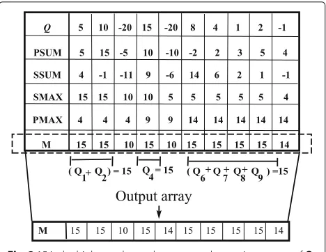
are three disjoint subsequences of maximum sum. The first consists of elements (x1,x2) with size 2; the second is represented by the element (x4) with size 1; the third con-sists of the elements (x6,x7, x8, x9) with size 4. All have sum equal to 15.
5 10 -20 15 -20 8 4 1 2 -1
X
(X + X ) =15
C
A B
1 2 4X =15 (X + 6 7 8 9X + X + X ) = 15
Fig. 1The three subsequences of maximum sum ofXwith the same sum [8]
Computational model
In this work we use the BSP/CGM parallel computation model [3, 15]. It consists of a set ofpprocessors, each hav-ing a local memory of size O(n/p), wherenis the problem size.
The BSP/CGM parallel computing model is a realis-tic model where special attention is given to minimize communications overheads. This model is particularly suitable nowadays in parallel machines where the overall computation speed is considerably larger than the overall communication speed.
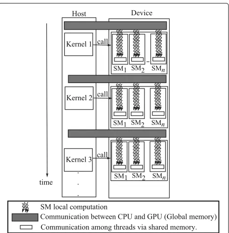
An algorithm in this model performs supersteps (a series of rounds), alternating well-defined local compu-tation and global communication phases, separated by a synchronization barrier. The cost of communication considers the number of rounds required. The implemen-tation of a BSP/CGM algorithm generally presents good results with performance similar to that predicted in its theoretical analysis [4]. Since the MPI library is designed for distributed memory environments, a BSP/CGM algo-rithm can be mapped into an MPI implementation using the message resources of this library. On the other hand, for the implementation of a BSP/CGM algorithm on a general purpose graphics processing unit (GPGPU) with CUDA, we need to establish the correspondence of com-putations and communications concepts in this environ-ment. In this context, the supersteps of the BSP/CGM model are represented by sequential invocations of each CUDA kernel. Furthermore, we associate the set of pro-cessors of the BSP/CGM model with the set of CUDA streaming multiprocessors (SMs). Figure 2 illustrates our suggestion for this process.
The extended solution
In 2004, Alves et al. [1] presented a BSP/CGM algo-rithm for the maximum subsequence sum problem. This algorithm is efficient, but like the previous solutions, it does not consider the existence of more than a subse-quence of maximum sum. Furthermore, since the algo-rithm works in a distributed environment, it performs a series of compressions that change the input sequence. This change causes difficulty in the search of more than one subsequence. On the other hand, using the ideas of the PRAM algorithm proposed by Perumalla and Deo [10], in this work we devise a new BSP/CGM paral-lel algorithm for this problem that uses the final output
to compute the shortest/longest maximum subsequences and the total number of disjoint maximum subsequences. Figure 3 illustrates an example of the output array of Perumalla and Deo’s algorithm [10]. Through the output array, we can find all disjoint subsequences of the max-imum subsequence sum problem. In this example, there are three disjoint maximum subsequences with differ-ent sizes. Next we presdiffer-ent new BSP/CGM algorithms to solve the 1D maximum subsequence sum problem, the shortest/longest maximum subsequences, and the total number of maximum subsequences.
The BSP/CGM algorithm for the maximum subsequence sum
We designed a BSP/CGM solution (see Algorithm 2) that solves the basic problem of maximum subsequence sum.
In the algorithm, the arraysPSUMandSSUMmean
pre-fix sum and sufpre-fix sum, respectively. We compute the
suffix maxima ofPSUMand prefix maxima ofSSUMand
store the results in the arraysSMAXandPMAX, respec-tively. The output of Algorithm 2 is an arrayMshown in Fig. 3.
Fig. 315 is the highest value and represents the maximum sum ofQ
[8]
Algorithm 2Maximum subsequence sum
Require:(1) A set ofPprocessors; (2) The numberiof each processorpi ∈ P, where 1 ≤ i ≤ P; (3) SequenceQofn
integers.
Ensure:(1) ArrayM[1. . .n] of integers with all disjoint subse-quences of maximum sum; (2)maxsumMaximum Subse-quence Sum.
1:PSUM←Prefix_Sum(P,Q)in parallel
2:SSUM← Suffix_Sum(P,Q)in parallel{Prefix sum opera-tion applied on the inverse arrayQ}
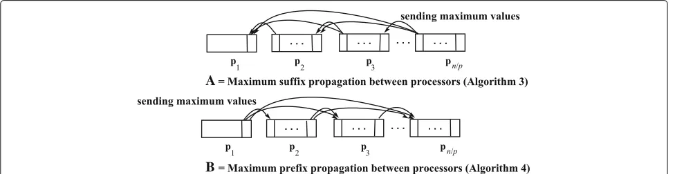
3:SMAX ← Maximum_Suffix_Propagation(P,PSUM) in parallel{Propagation of maximum values from end to the beginning}
4:PMAX ← Maximum_Prefix_Propagation(P,SSUM) in parallel{Propagation of maximum values from beginning to the end.}
5:Processorp1 sendsn/p elements of each arrayQ,PSUM,
SSUM,SMAXandPMAXto each processorpi∈P.
6:Each processorpiin parallelobtains the local arrays: LocalMS←PMAX(n/p)−SSUM(n/p)+Q(n/p) LocalMP←SMAX(n/p)−PSUM(n/p)+Q(n/p) LocalM←LocalMS(n/p)+LocalMP(n/p)−Q(n/p)
7:Each processorpisends arrayLocalM in parallelto
proces-sorp1, which computes arrayM:
M=[LocalMp11,. . .,LocalMp1n/p,. . .,LocalMpp1,. . .,
LocalMppn/p]
8:maxsum←Maximum_Reduction(P,M)in parallel
Two operations are performed in the algorithms “Maximum_Suffix_Propagation and Maximum_Prefix_ Propagation” (they are called from Algorithm 2), both consisting of a maximum propagation. The first opera-tion occurs in the local array of each processor. In this case, higher values are propagated, replacing the smaller values. The replacement is performed until a (new) higher value is found, which then starts a new maximum propagation, as illustrated in Fig. 4. The second operation occurs between each processor and the greater value of the maximum values of the subsequent/precedent pro-cessors, as illustrated in Fig. 5. For the sake of simplicity,
we present only the “Maximum_Suffix_Propagation”
(Algorithm 3). The main difference of the algorithms is the direction of propagation. For the complete
explana-tion about the variables (PSUM, SSUM,PMAX, SMAX,
LocalMP,LocalMS, andLocalM), please see [10].
Algorithm 3Maximum_suffix_propagation Require:(1) ArrayPSUM[ 1. . .n] of integers.
Ensure:(1) ArraySMAX[ 1. . .n] of integers.
1:Processorp1sendsn/pelements ofPSUMto each processor
pi∈P.
2:In each processorpi, an operation of maximum propagation
is performed inPSUM(n/p). The operation is initiated in the element of index(n/p)×(i)and runs until the element of index(n/p)×(i−1). At the end, the maximum element is in the first position.
3:Finally, an operation of maximum propagation is performed between each processor pi and the maximum element
among all the maximum elements of the processors pk,
wherek>i.
Correctness and complexity
Besides the fact that we use onlypprocessors, the steps of our main BSP/CGM algorithm can be easily derived from the PRAM algorithm [10]. Using BSP/CGM parallel prefix algorithms, steps 1 and 2 can be computed usingp proces-sors in O(n/p)time and O(logp)communication rounds. For steps 3 and 4, we use Algorithm 3, requiring p pro-cessors with O(n/p) time and O(logp) communication rounds. Steps 5 to 7 can be computed usingpprocessors with O(n/p)time and a constant number of communica-tion rounds. Finally, using BSP/CGM parallel maximum
reduction algorithm, step 8 is computed using p
pro-cessors with O(n/p) time and O(logp) communication rounds. Therefore, Algorithm 2 computes the maximum subsequence sum correctly usingpprocessors in O(n/p)
time with O(logp)communication rounds.
The BSP/CGM algorithms for the related problems
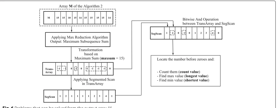
We also developed BSP/CGM algorithms to solve three problems related to the maximum subsequence sum, that is, (1) the longest maximum subsequence sum, (2) the shortest maximum subsequence sum, and (3) the number of disjoint subsequences of maximum sum. The output of Algorithm 2 is the starting point of these three algorithms. For simplicity, the strategies of these algorithms are listed in only one algorithm, represented here by Algorithm 4.
First, using the arrayTransArray, we mark all the ele-ments of arrayMthat are equal tomaxsum.
Then, we compute the array SegScan that stores the
A
B
Fig. 4Local operations
Since we are searching the regions inMwhere we have maximum values, we perform a bitwise operation with the SegScanandTransArrayarrays. This operation changes theSegScanarray and all the elements in this array that do not correspond to the elements inMthat represent the maximum subsequences become equals 0. The subarrays inSegScanthat are not null are enumerated and represent the maximum sum subsequences.
The maximum subsequences and their respective sizes are easily found using parallel BSP/CGM prefix/suffix sum, reduction, and other basic algorithms.
Correctness and complexity
In order to find the maximum subsequences in M, we
use basic BSP/CGM algorithms for prefix/suffix sum, Segmented Scan and Bitwise And Operation. Efficient BSP/CGM parallel algorithms for these problems can be found in Dehne at al. [4]. Figure 6 illustrates the relation-ship among the internal routines listed by Algorithm 4 and
the solutions that can be drawn from them. The starting point is the output of Algorithm 2. Algorithm 4 computes correctly and returns the three expected values.
Using BSP/CGM reduction algorithms, the internal rou-tines of Algorithm 4 associated with the sizes of maximum
subsequence sum can be computed usingpprocessors in
O(n/p)time and O(logp)communication rounds. Hence, the combination of Algorithms 2 and 4 yields the solution in O(n/p)time with O(logp)communication rounds.
Results
The main advantage of using the BSP/CGM model to design parallel algorithms is that when implemented in real environments, they have an expected behavior as stated by their theoretical analysis. In this work, we imple-mented our algorithm using both distributed and shared memory environments. The results showed that the exe-cution times were compatible with those foreseen by the theoretical analysis.
A
B
Fig. 6Problems that can be solved from the output arrayM
Algorithm 4Related problems
Require: (1) ArrayM[ 1. . .n] of integers (Output from Algo-rithm 2) ; (2) The value of maximum sum (maxsum) (Output from Algorithm 2).
Ensure: (1) Thelongest= size of the longest maximum sub-sequence sum ; (2) Theshortest = size of the shortest maximum subsequence sum ; (3) Thecount= number of disjoints subsequences of maximum sum.
1: Use the set of processorsPto obtain the transformed array
TransArray[ 1. . .n], as follows:
2: for∀1≤i≤nin parallel do
3: if (M[i]=maxsum) then
4: TransArray[i]← −1 {All bits are set to 1 (two’s complement representation)}
5: else
6: TransArray[i]←0 {All bits are set to 0}
7: end if
8: end for
9: SegScan[ 1. . .n]←Segmented_Scan(M[ 1. . .n])in par-allel
10: SegScan[ 1. . .n]←SegScan[ 1. . .n] &TransArray[ 1. . .n]
in parallel{Bitwise And Operation}
11: count←0
12: shortest←MAX_VALUE
13: longest←MIN_VALUE
14: for∀(SegScan[i]=0 andSegScan[i+1]=0)in parallel do
15: count ← count+1 {Apply a Parallel Sum Reduction
Algorithm}
16: shortest ← min(shortest,SegScan[i]){Apply a Par-allel Minimum Reduction Algorithm}
17: longest ←max(longest,SegScan[i]){Apply a Paral-lel Maximum Reduction Algorithm.}
18: end for
We used a 32-node cluster of workstations and the mes-sage passing interface (MPI) to implement our algorithms in a distributed memory environment. The shared mem-ory environment was tested with several configurations. The open multi-processing (OpenMP) implementation used workstations with 2/4/6 cores. The GPGPU/CUDA version of the algorithm was implemented using one GPU and four GPUs. Previous works have shown the good per-formance of BSP/CGM algorithms when implemented on clusters of workstations [1]. In this work, we use four different computing systems with shared memory, which allow us to confront our shared memory implementations against a similar distributed memory implementation. For comparison purpose, the speedups were computed using as reference the time spent by the sequential implementa-tion in a host of the computing system were the respective parallel algorithms where executed. All the implementa-tions showed competitive speedups.
Computational resources
We have run the experiments on five different computing systems (Table 1), with shared and distributed memory. Four of those computing systems (CS-1, CS-2, CS-3, and CS-5) use shared memory and have at least one CUDA GPU (one of them has four identical GPUs) with differ-ent specifications, which allow us to check the consistency
Table 1Platforms—general specs
ID Processor Clock Cores/threads RAM/cache Linux/dist./GCC
CS-1 Xeon E5-2620 2.00 6/12 16/15 CentOS 7.2/3.10.0 / 4.8.5
CS-2 Core i7-3770 3.40 4/8 8/8 Ubuntu 12.04/3.2.0-37/4.6.3
CS-3 Core2 Quad Q9550 2.83 4/4 4/6 Ubuntu 15.04/3.19.0-15/4.9.2
CS-4 Xeon E5620 2.40 4/8 8/12 CentOS 6.8/2.6.32/4.4.7
Table 2Platforms—CUDA specs
ID GPU (NVidia) # GPUs RAM # SMs Cuda cores Clock GPU arch/SDK
CS-1 GTX TITAN Black 4 6 15 2880 889 3.5/7.5
CS-2 GTX 680 1 2 8 1536 1006 3.0/4.2
CS-3 GTX 460 v2 1 1 7 336 778 2.1/7.5
CS-5 GT 720M 1 2 2 192 797 2.1/7.5
and performance of our algorithms using shared memory environment. One of the computing systems (CS-4) is a cluster of 32 nodes connected with a Myrinet switch using 10 Gb/s Ethernet.
The technical specifications of the computing systems are depicted in Tables 1, 2, and 3. All the processors use 64–bit architecture. The clock frequency is given in GHz, the cache memory in MB, and the RAM memory in GB.
Execution methodology
We used randomly generated data for input arrays vary-ing from 220to 229 elements. For each input, we ran the experiment 20 times and measured the average running time. To make sure that such an average is representative of the expected value, we apply the Shapiro-Wilk [14] sta-tistical test to the 20 times obtained, and we tolerate the discarding of five values, thereby resulting in a minimum of 15 and a maximum of 20 valid values to compute the average. The result of the statistical test (Pvalue) has to be greater thanα > 0.05, so that we can assert with signifi-cance level of 5 % that the sample derives from a normal population. In case the statistical test givesα ≤0.05, the sample is discarded and new running times are collected for that input.
The algorithms were tested in the distributed memory environment CS-4 using MPI. In this environment, we can specify the number of nodes and their respective proces-sors to be allocated for the execution, in the form ofNX:
PY (Xnodes, withY processors each).The configuration
N32 : P8 means that we used 32 nodes of the cluster,
each with 8 threads, with a total of 256 MPI processes. We executed our algorithm with the following configura-tions:N16 :P1,N16 :P2,N16 :P4,N16 :P8,N32 :P1,
N32 :P2,N32 :P4, andN32 :P8.
In the shared memory environment, we used OpenMP and CUDA. The CUDA implementation of the algorithms were executed on CS-1, CS-2, CS-3, and CS-5 platforms. In the CS-1 platform, we also varied the number of GPUs, where we used 1, 2, and 4 GPU configurations. The OpenMP implementation was executed in all platforms.
Table 3Platforms—MPI specs
ID Cluster # Nodes/threads # MPI proc. mpicc Comm.
CS-4 Cluster Rocks 6.0 (Mamba)
46/8 368 4.4.7 Myrinet
10 Gb/s
We tested the OpenMP implementation with different numbers of threads. In all platforms, we used 1, 2, and 4 threads, while we also tested with 8 threads in the CS-1, CS-2, and CS-4 and with 12 threads in the CS-1.
A sequential version of the algorithm, with the related problems, was implemented using C. This implementa-tion was executed in all platforms. The speedups of the parallel versions were computed using the execution time of the sequential implementation of the algorithms in the respective platform as reference.
Due to the exponential variation of the input values (with 220 ≤ n ≤ 229), all the curves use the logarithmic scale (base 2) as the horizontal axis. Vertical axis (runtime and speedup) uses logarithmic scale (base 10) for better presentation and visualization.
Results
Now we present the results that were obtained using the five computing systems. First we present the execution times of the sequential version of the algorithms. As we stated above, we implemented it on all platforms in order to compute the respective speedup in each computer system.
Sequential implementation
We developed a sequential version of the Perumalla and Deo parallel algorithm [10], and we extended the sequen-tial version for solving the related problems. The complete algorithm has O(n)time complexity. It was implemented on all platforms.
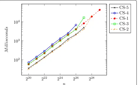
Table 4Running times (milliseconds) of sequential implementation
n CS-5 CS-4 CS-1 CS-3 CS-2
220 35.811 71.143 57.314 59.100 31.517
221 69.225 141.295 110.836 114.250 62.986
222 135.859 283.747 219.730 225.275 126.487
223 284.376 636.522 531.464 502.136 250.795
224 543.696 1305.605 1063.938 1005.549 501.978
225 1225.326 2492.813 2114.072 2005.769 1004.222
226 2186.893 6825.944 4105.771 4012.655 2022.964
227 4985.319 – 8272.913 16,682.755 4030.542
228 – – 18,931.466 – 20,327.877
229 – – 42,466.062 – –
Figure 7 and Table 4 show the behavior of the algorithm on each platform. We observe that when the input size reaches the resource limits of the platform, the execution results stop obeying the expected curve of the execution times. This phenomenon is calledThrashing[5]. It occurs because of the constant paging, which degrades the com-plete system performance. In some cases, it freezes the system. In some tests, the operating system killed the pro-cess and we could not collect the result. In these cases, if the time was collected, it would be equivalent or worse than that when the thrashing phenomenon occurs.
MPI implementation
We developed a version of the BSP/CGM algorithms for distributed memory. This version was implemented with MPI and uses the resources of MPI which includes a number of library functions for communication and syn-chronization among all members of a process group.
The sequence is divided inpsubsequencessi, 1≤i≤p
of sizen/p. Each processorpi(1≤i≤p)receives the
sub-sequencesiand compute the algorithm locally. The partial
solutions (boundaries) are exchanged using built-in func-tions of the MPI. The details of the code can be seen in https://github.com/rodrigogbranco/extendedmss.
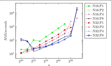
Fig. 8CS-4 running times (milliseconds) of MPI implementation
Figure 8 and Table 5 show the average execution times. We executed the MPI implementation using 16 and 32 nodes with different numbers of threads.
We can see that when the input is not big enough, there is a communication overhead. This depends on the num-ber of used nodes and impacts the execution times. After a given size of the input, the execution times present a linear behavior (in each processor the time complex-ity is O(n/p)). When the size of the input is too big, the thrashing phenomenon occurs again. In some cases, such asN16 : P1, the operating system/cluster manage-ment aborted the application with input sizes ofn = 228 andn=229.
OpenMP implementations
Using the ideas of the distributed memory BSP/CGM algorithms that were implemented with MPI, we imple-mented them in a shared memory environment using OpenMP (Table 6 and Fig. 9). The main difference was that the message exchange among the processes (threads) was done in the memory of the workstations. We used the OpenMP directives to create and eliminate threads and shared arrays and schedule functions. When supported by the compilers, we used directives for array reduction. The details of the code can be seen in https://github.com/ rodrigogbranco/extendedmss.
Table 5CS-4 running times (milliseconds) of MPI implementation
n N16:P1 N16:P2 N16:P4 N16:P8 N32:P1 N32:P2 N32:P4 N32:P8
220 10.730 11.403 9.788 91.368 11.597 19.765 21.263 119.741
221 21.403 15.286 12.880 83.876 16.562 21.004 18.488 79.335
222 99.957 23.938 18.761 16.064 24.395 25.461 21.225 23.279
223 82.786 40.277 29.675 21.406 45.941 33.450 26.846 28.399
224 175.851 75.340 51.073 33.305 82.706 52.493 38.760 33.242
225 357.882 139.970 90.844 53.800 146.140 93.536 59.839 46.379
226 748.831 263.430 161.765 100.714 263.629 164.268 93.531 66.719
227 1546.020 559.685 307.145 171.782 555.407 288.917 170.073 111.906
228 – 1331.303 2356.562 314.681 854.059 426.578 317.116 203.811
229 – – – 24,301.072 – 4174.692 – 17,766.883
Multi-GPU implementation
One of the goals of this work is to show that the BSP/CGM model is suitable for designing parallel algorithms for dis-tributed and shared memory alike. Besides that, we also want to show that the BSP/CGM algorithms can be imple-mented in GPGPUs with good speedups. In order to verify the efficiency of the algorithm in the GPGPUs environ-ment, we tested it with four different configurations. One of the configurations is a multi-GPGPU with four devices (GPUs).
Differently from the MPI and OpenMP environments, the implementation of a BSP/CGM algorithm using CUDA/GPGPU has a higher level of complexity. For this reason, in this section, we choose to present a step by step description of the parallel implementation of the 1D max-imum subsequence sum and the related problems using CUDA/GPGPU. The details of the code can be seen in https://github.com/rodrigogbranco/extendedmss.
Figure 2 shows how we can map a BSP/CGM algorithm onto a GPGPU. The computation rounds are done by the SMs. The computation is executed by sets of blocks of threads. Each thread runs a copy of the same program in the GPGPU (kernel function).
We implemented our algorithm in the GPGPU using CUDA. With CUDA, a kernel function specifies the code to be executed by all threads in a parallel step (compu-tation round). When a kernel is called, or launched, it is executed as a grid of thread blocks in parallel. Each thread block is scheduled separately for a SM. Threads within the same block are organized in units of 32 threads, called warps [13]. To maximize even further the performance, CUDA uses different memory types. Each memory is used for different purposes. The shared memory, for example, is used to exchange data between threads within a CUDA block [13]. When a kernel finishes its computation, we have a synchronization. After that, we have a new round or the program finishes.
First we describe the steps of our implementation that uses only one GPGPU.
As shown in Table 7, we used the Thrust Library [6] extensively, including the device vector (using
thrust::device_vector) and host vector (usingthrust::host_ vector) when implementing Algorithms 2 and 4 with CUDA. These types of vectors were chosen to simplify the use of optimized Thrust functions, and also the memory transfers between device-host and vice-versa.
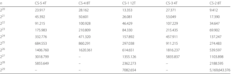
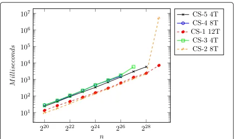
Table 6Running times (milliseconds) of OpenMP implementation
n CS-5 4T CS-4 8T CS-1 12T CS-3 4T CS-2 8T
220 23.917 28.162 13.353 27.371 9.412
221 45.392 50.601 26.081 53.049 17.390
222 91.215 100.928 46.429 107.229 34.647
223 175.983 210.809 84.330 215.435 69.902
224 332.776 471.320 157.892 457.911 137.247
225 684.553 860.291 297.038 911.215 274.483
226 1406.760 1620.361 614.651 1816.237 539.597
227 3018.799 – 1355.126 5835.837 1103.898
228 5855.649 – 2362.273 – 2188.595
Fig. 9Running times (milliseconds) of OpenMP implementation
Now we detail the CUDA implementation steps of Algo-rithms 2 and 4.
Steps 1 and 2 (Sum of Prefixes and Sum of Suf-fixes): In order to solve steps 1 and 2, we used
thrust::inclusive_scan. We used the reverse iterator of
thrust::device_vectorto iterate and compute sum of suf-fixes transparently.
Steps 3 and 4 (Maximum Suffix Propagation
and Maximum Prefix Propagation): These steps
follow the same idea of steps 1 and 2 but using
thrust::maximumrather than the defaultthrust::plusused onthrust::inclusive_scan.
Steps 5–9: To build the output arrayM, some arithmetic operations involving the initial four arrays were needed. For that, we used the functionthrust::transformto operate individually on each element of array.
Table 7Thrust and CUDA functions used by Algorithms 2 and 4
Algorithm Steps Thrust function
Algorithm 2 (1) PSUM (2) SSUM thrust::inclusive_scan
Algorithm 2 (1) PSUM (2) SSUM thrust::for_each(to correct borders - multi-GPUs)
Algorithm 2 (3) SMAX (4) PMAX thrust::inclusive_scan
Algorithm 2 (3) SMAX (4) PMAX thrust::for_each(to correct borders - multi-GPUs )
Algorithm 2 (7) Compute array M thrust::transform
Algorithm 2 (8) Maximum reduction thrust::reduce
Algorithm 4 (2) Transformation thrust::for_each
Algorithm 4 (7) Segmented scan thrust::inclusive_scan_by_key
Algorithm 4 (8) Bitwise and operation thrust::transform,thrust::find
Algorithm 4 (8) Bitwise and operation thrust::for_each(to correct borders - multi-GPUs)
Algorithm 4 (12) Find related solutions findRelatedSolutions (Custom Kernel)
– Synchronization __syncthreads(threads)
– Synchronization cudaDeviceSynchronize
(blocks and device-host)
Step 10: To solve this step, we usedthrust::reduceusing
thrust::maximum.
At the beginning of Algorithm 4, we built the TransAr-ray usingthrust::for_each, with a custom function oper-ation to manipulate the individual elements. So, in that
function we passed the maxsum and, if the element
was equal to it, then it would receive –1 value and
0 otherwise. We built a new array using TransArray,
applying theSegmented_Scanoffered by Thrust through
thrust::inclusive_scan_by_key(see Fig. 6).
With bothTransArrayandSegScanready, we applied
the bitwise and operation (&) usingthrust::transformand
thrust::bit_and. Finally, we built a CUDA kernel to pro-cess the last part of Algorithm 4 (quantity of maximum subsequence sum, longest subsequence, and shortest sub-sequence).
Our CUDA implementation with more than one GPU works on the same host. Therefore, in order to man-age each GPU transparently, we used OpenMP, and each thread was responsible for managing its own GPU. It is important to note that here OpenMP is being used only to manage the GPUs and run the
synchroniza-tion among them through the funcsynchroniza-tion
cudaDeviceSyn-chronize() (GPU-host synchronization), followed by the
directive #pragma omp barrier (synchronization among
threads).
When the algorithm was implemented in a multi-GPU system, we had to take care of some details. After the end of some steps of a GPU we need to do some extra work, since each GPU works with an/(#gpus) partition of the array M[ 1. . .n]. The same occurs for the arraysPSUM
andSSUM. After the GPU finalizes each of steps 1 and 2 of Algorithm 2, they need to correct their array borders. Those corrections can be done by using the shared mem-ory of the host with the functionthrust::for_each. At the
end of steps 3 and 4, the first element of arraysPMAX
and SMAX may need to be corrected too. This also is
done with the functionthrust::for_each. Algorithm 4 uses the function thrust::for_each after step 8 to correct the
Table 8Running times (milliseconds) of CUDA implementation
n CS-1 4GPUs CS-1 2GPUs CS-1 1GPU CS-3 CS-5 CS-2
220 9.033 10.338 4.040 4.701 19.220 2.650
221 15.794 12.300 5.194 7.839 36.470 4.310
222 15.661 14.138 7.456 14.254 71.342 7.662
223 15.053 16.320 11.999 27.1798 139.110 14.505
224 16.036 17.480 20.913 53.415 304.978 28.348
225 23.632 31.100 39.653 – 573.287 56.360
226 30.764 56.451 76.051 – – –
227 55.126 92.363 149.896 – – –
228 103.174 178.439 – – – –
229 204.072 – – – – –
borders too. In the last step, each GPU sends its three values (quantity of maximum subsequence sum, longest subsequence, and shortest subsequence) to the host that will compute the final solution.
Now we describe some strategies that we used in the implementation. To make a better use of the GPU, two techniques were utilized: persistent threads and efficient communication among SPs. A kernel was launched with the number of blocks of threads as a multiple of the amount of blocks executed concurrently in each SM. Since a SM can process one or more blocks of threads simulta-neously, we avoid blocks of threads staying in the schedul-ing queue. As a consequence, each block of threads stay persistent and can operate on more than one part of the input, when this input is larger than the grid of blocks of the kernel. The multiplicity of the amount of blocks of threads selected was two times the number of SMs. This choice was based on the experiments using the pro-filenvprof, that obtained the best result, achieving 95 % of occupancy.
The use of efficient communication among the SPs is related to the SIMD functionality offered by the latest ver-sions of GPUs. This functionality allows that SPs within an SM communicate through the shared memory and
Fig. 11Best running time (milliseconds) of each implementation
without synchronization, simply using registers. A sec-ond implementation was created for older versions of GPUs (capability <3.0) by using communication through the shared memory and synchronizations.
We also exploited the memory hierarchy of the GPU by moving data from global memory to shared memory (and registers) so as to promote coalesced access and avoid the high costs associated with global memory. The thread’s resource utilization was kept low, thus permitting more threads to be used per block and a full occupation the GPU SMs.
Finally, the optimized thrust::reduce was used to per-form the reductions between blocks, finding the results for a single GPU. Each GPU sent its results to host for final reductions. It was possible to take advantage of memory coalescing and thereby achieve good performance results. The running times of the CUDA GPU implementations are presented in Fig. 10 and Table 8. As in the MPI imple-mentation, it is possible to observe some overhead for the first inputs when more than one GPU is used in the execu-tion. However, starting from the input sizen=224, we can note that this overhead decreases significantly. A curiosity relative to the other implementations is the fact that the
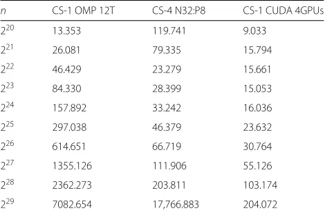
Table 9Best running time (milliseconds) of each implementation
n CS-1 OMP 12T CS-4 N32:P8 CS-1 CUDA 4GPUs
220 13.353 119.741 9.033
221 26.081 79.335 15.794
222 46.429 23.279 15.661
223 84.330 28.399 15.053
224 157.892 33.242 16.036
225 297.038 46.379 23.632
226 614.651 66.719 30.764
227 1355.126 111.906 55.126
228 2362.273 203.811 103.174
Fig. 12Speedups—parallel/sequential in the same platform
thrashing phenomenon does not occur here. The expla-nation for this is that the memory of the GPUs is stressed in this situation and, on reaching the limit of its capacity, the GPU driver informs the impossibility to continue and the execution is aborted. Therefore, the main memory, in those positions used by the application, is not paged and, for this reason, the thrashing phenomenon is not verified.
Best running times of each implementation and speedups Figure 11 and Table 9 present the best running times for each of the implementations (OpenMP, MPI, and CUDA). Since the configurations of the Platform CS-1 is a 4-GPUs system, we can already expect that the best running times of the implementations occur in this envi-ronment. The results show the scalability of the algorithm and the implementations presented: the addition of more threads/nodes/GPUs tends to present superior results.
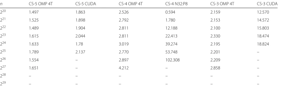
In order to show the speedups, we computed them with respect to each platform. Figure 12 and Tables 10 and 11 present the speedups relative to the sequential and parallel implementation executed in the same platform. We can see that the OpenMP implementations, in gen-eral, tend to preserve the speedup with little variation, as well as the CUDA implementations with GPUs cards of
lower performance. The exceptions are implementations CS-1 CUDA 4GPUs and CS-4 N32:P8, for which we can observe speedups of approximately 102 times for the MPI implementation and approximately 208 times for the multi-GPU CUDA version.
The platforms and equipments available were not suf-ficient to discover how many MPI processes (nodes and processes per node) would be sufficient to reach the speedup of the Multi-GPU implementation, due to the limitations in the submission of jobs to the cluster.
All source codes of the implementations can be found at https://github.com/rodrigogbranco/extendedmss.
Conclusions
There are good sequential and parallel solutions to the problem of maximum subsequence in the literature. How-ever, they consider only one subsequence of maximum sum for each input sequence. Therefore, to circumvent this shortcoming, we developed BSP/CGM parallel algo-rithms that consider the simultaneous existence of more than one maximum subsequence sum.
Furthermore, our algorithms can find solutions for three new related problems: the maximum longest subsequence sum, the maximum shortest subsequence sum, and the number of disjoints subsequences of maximum sum. To the best of our knowledge, there are no parallel algorithms for these related problems. The algorithms work for shared and distributed memory and were implemented using a multi-GPU/CUDA, OpenMP, and MPI.
In the design of our algorithms, we use the BSP/CGM model of parallel computing. It is well known that this model is suitable for designing parallel algorithms for distributed memory platforms. In this work, we showed good results when mapping our BSP/CGM algorithms to shared memory platforms. The implementations of the proposed algorithms were shown to be efficient and have good speedup results, as confirmed by experimen-tal results. The running times of the MPI and CUDA
Table 10CS-4 running times (milliseconds) of MPI implementation
n CS-5 OMP 4T CS-5 CUDA CS-4 OMP 4T CS-4 N32:P8 CS-3 OMP 4T CS-3 CUDA
220 1.497 1.863 2.526 0.594 2.159 12.570
221 1.525 1.898 2.792 1.780 2.153 14.572
222 1.489 1.904 2.811 12.188 2.100 15.803
223 1.615 2.044 2.811 22.413 2.330 18.474
224 1.633 1.78 3.019 39.274 2.195 18.824
225 1.789 2.137 2.770 53.748 2.201 –
226 1.554 – 2.897 102.308 2.209 –
227 1.651 – 4.212 – 2.858 –
228 – – – – – –
Table 11Speedups—parallel/sequential in the same platform - II
n CS-2 OMP 8T CS-2 CUDA CS-1 OMP 12T CS-1 CUDA 4GPUs
220 3.348 11.893 4.292 6.344
221 3.621 14.610 4.249 7.017
222 3.650 16.508 4.7322 14.030
223 3.587 17.289 6.302 35.305
224 3.657 17.707 6.738 66.345
225 3.658 17.817 7.117 89.454
226 3.749 – 6.679 133.460
227 3.651 – 6.104 150.070
228 9.288 – 8.014 183.489
229 – – 5.995 208.092
implementations are several times better than the sequen-tial solution in the respective platform. Furthermore, the CUDA implementation can easily be implemented with one or several GPUs.
The proposed algorithms usepprocessors and require
O(n/p)parallel time with a constant number of commu-nication rounds for the algorithm of the maximum sub-sequence sum and O(logp)communication rounds, with O(n/p)local computation per round, for the algorithms of the related problems.
The results obtained lead us to believe that the posed algorithms are scalable, since the addition of pro-cessing elements in the platforms has not yet reached the saturation point. This means that the addition of threads/nodes/processors/GPUs in the respective plat-forms can increase the speedup significantly. Unfortu-nately, the available platforms do not allow us to reach the saturation point, since problems related to the limitation of the available resources have appeared, such as Thrash-ing and the elimination of the process by the operating system.
The results also showed the efficiency of the multi-GPU version, even for large sizes of the input data. Our
implementation supported up to 229elements with good
running times, that is, supported more than 500 million elements as the input of the problem.
As future work, we intend to extend the multi-GPU implementation to solve the maximum sum subarray problem, with more than one dimension (2D and 3D problems). We also intend to compute all the maximal subsequences in a given interval.
Acknowledgements
The authors thank FUNDECT, FAPEG, FAPESP (2013/26644-1), CNPq (482736/2012-7, 302620/2014) and Capes/PVE 002/2012 and NVIDIA. Thanks are also due to the anonymous referees for their comments and suggestions.
Authors’ contributions
ACL, RAG, ENC, WSM, and SWS worked on the model proposal and the design, correctness, and complexity of the algorithms. RAG, ACL, RGB, and SF worked
on the implementation details of the algorithms. All authors read and approved the final manuscript.
Competing interests
The authors declare that they have no competing interests.
Author details
1Faculdade de Computação da Universidade Federal de Mato Grosso do Sul, Cidade Universitária, C.P: 549 Campo Grande, MS, Brasil.2Instituto de Informática da Universidade Federal de Goiás, Campus Samambaia, C.P: 131 Goiânia, GO, Brasil.3IME, Universidade de São Paulo, Rua do Matão, São Paulo, Brasil.
Received: 8 October 2015 Accepted: 6 September 2016
References
1. Alves CER, Cáceres EN, Song SW (2004) BSP/CGM algorithms for maximum subsequence and maximum subarray. In: Recent Advances in Parallel Virtual Machine and Message Passing Interface, volume 3241 of Lecture Notes in Computer Science. Springer, Berlin Heidelberg. pp 139–146 2. Bentley J (1984) Programming pearls: algorithm design techniques.
Commun ACM 27(9):865–873
3. Dehne F, Fabri A, Rau-chaplin A (1994) Scalable parallel computational geometry for coarse grained multicomputers. Int J Comput Geom 6:298–307
4. Dehne F, Ferreira A, Cáceres EN, Song SW, Roncato A (2002) A efficient parallel graph algorithms for coarse grained multicomputers and BSP. Algorithmica 33(2):183–200
5. Denning PJ (1968) Thrashing: its causes and prevention. In: Proceedings of the December 9-11, 1968, Fall Joint Computer Conference, Part I. AFIPS ’68 (Fall, part I). ACM, New York. pp 915–922. doi:10.1145/1476589.1476705 6. Hwu W-MW (2011) GPU Computing Gems Jade Edition. 1. Morgan
Kaufmann Publishers Inc, San Francisco
7. Ladner RE, Fischer MJ (1980) Parallel prefix computation. J ACM 27(4):831–838
8. Lima AC, Branco RG, Cáceres EN, Gaioso RA, Ferraz S, Martins WS, Song SW (2015) Efficient BSP/CGM algorithms for the maximum subsequence sum and related problems. Int Conf Comput Sci ICCS:2754–2758 9. Marcus SL, Brumell SL, Pfeifer CG, Finlay BB (2000) Salmonella
pathogenicity islands: big virulence in small packages. Microbes Infect 2(2):145–156
10. Perumalla K, Deo N (1995) Parallel algorithms for maximum subsequence and maximum subarray. Parallel Process Lett 5:367–363
11. Qiu K, Akl SG (1999) Parallel maximum sum algorithms on interconnection networks. Technical report, Queens University Dept. of Com., Ontario 12. Ruzzo WL, Tompa M (1999) A linear time algorithm for finding all maximal
scoring subsequences. In: Proceedings of the 7th International Conference on Intelligent Systems for Molecular Biology. AAAI Press. pp 234–241
13. Sanders J, Kandrot E (2011) CUDA by example: an introduction to general-purpose GPU programming. Ed 1. Addison-Wesley, USA 14. Shapiro SS, Wilk MB (1965) An analysis of variance test for normality
(complete samples). Biometrika 3–4(52):591–611
15. Valiant LG (1990) A bridging model for parallel computation. Commun ACM 33:103–111