Complete trajectory reconstruction from sparse mobile phone data

R E G U L A R A R T I C L E

Open Access

Complete trajectory reconstruction from

sparse mobile phone data

Guangshuo Chen

_{, Aline Carneiro Viana}

_{, Marco Fiore}

_{and Carlos Sarraute}

*_{Correspondence:}

[email protected] 1_{INRIA, Université Paris-Saclay,} Palaiseau, France

2_{École Polytechnique, Université} Paris-Saclay, Palaiseau, France Full list of author information is available at the end of the article

Abstract

Mobile phone data are a popular source of positioning information in many recent studies that have largely improved our understanding of human mobility. These data consist of time-stamped and geo-referenced communication events recorded by network operators, on a per-subscriber basis. They allow for unprecedented tracking of populations of millions of individuals over long periods that span months. Nevertheless, due to the uneven processes that govern mobile communications, the sampling of user locations provided by mobile phone data tends to be sparse and irregular in time, leading to substantial gaps in the resulting trajectory information. In this paper, we illustrate the severity of the problem through an empirical study of a large-scale Call Detail Records (CDR) dataset. We then propose Context-enhanced Trajectory Reconstruction, a new technique that hinges on tensor factorization as a core method to complete individual CDR-based trajectories. The proposed solution infers missing locations with a median displacement within two network cells from the actual position of the user, on an hourly basis and even when as little as 1% of her original mobility is known. Our approach lets us revisit seminal works in the light of complete mobility data, unveiling potential biases that incomplete trajectories obtained from legacy CDR induce on key results about human mobility laws, trajectory uniqueness, and movement predictability.

Keywords: Human mobility; Mobile phone dataset; Data enrichment; Seamless trajectory reconstruction; Location predictability; Trajectory unicity

1 Introduction

Over the past ten years, the proliferation of mobile devices indirectly fuelled many origi-nal studies on human mobility, as mobile phone data collected by network operators have become an invaluable source of information about individual movement patterns at scale. Data extracted from mobile communications have supported many breakthroughs [1,2], including seminal works demonstrating that individual movements are regular [3] and predictable [4], as well as unique [5]. Mobile phone data have allowed unveiling major patterns in human movements, such as home-work commuting [6], or frequent and re-current motifs [7]. The novel understanding of individual movements enabled by network operator data has facilitated innovation in,e.g., transportation systems [8], urban planning [9], communication infrastructure deployment [10,11], and epidemics control [12].

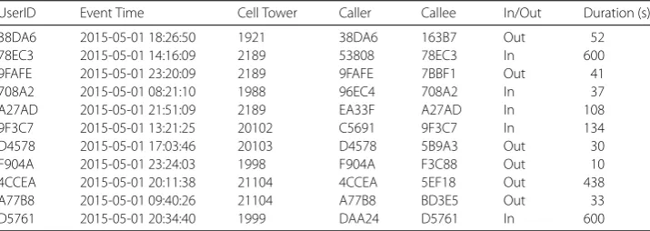
Call Detail Records(CDR) are the current de-facto standard for mobile phone data used in human mobility studies. As illustrated in Table1, CDR are logs of events generated

Table 1 The sample of CDR dataset. In this case, each CDR entry describes a voice call. All user identifiers and cell tower ids are coded to hide personal information. The GPS location of the cell towers is provided in the data source

UserID Event Time Cell Tower Caller Callee In/Out Duration (s)

38DA6 2015-05-01 18:26:50 1921 38DA6 163B7 Out 52

78EC3 2015-05-01 14:16:09 2189 53808 78EC3 In 600

9FAFE 2015-05-01 23:20:09 2189 9FAFE 7BBF1 Out 41

708A2 2015-05-01 08:21:10 1988 96EC4 708A2 In 37

A27AD 2015-05-01 21:51:09 2189 EA33F A27AD In 108

9F3C7 2015-05-01 13:21:25 20102 C5691 9F3C7 In 134

D4578 2015-05-01 17:03:46 20103 D4578 5B9A3 Out 30

F904A 2015-05-01 23:24:03 1998 F904A F3C88 Out 10

4CCEA 2015-05-01 20:11:38 21104 4CCEA 5EF18 Out 438

A77B8 2015-05-01 09:40:26 21104 A77B8 BD3E5 Out 33

D5761 2015-05-01 20:34:40 1999 DAA24 D5761 In 600

ing mobile communications, such as voice calls, text messages, and possibly mobile data traffic sessions, which are collected for billing purposes [2]. Those events are associated with individual mobile devices and are time-stamped and geo-referenced, which makes CDR an obvious proxy for the trajectories of the mobile network subscribers. Interest-ingly, CDR encompass huge populations (e.g., millions of users) over large (e.g., citywide or nationwide) geographic regions, and cover long periods (e.g., months or years): they thus enable human mobility investigations at unprecedented scales.

A drawback of CDR-based trajectories (or simply trajectories hereafter) is that they are often largely incomplete. As a matter of fact, telecommunication events are punctual and provide information at specific time instants, which are also sparse and irregularly distributed in time. Thus, CDR offer a very partial view of the overall mobility of each user, with substantial continuous periods where location information is entirely absent [13]. From a research standpoint, the reduced completeness of CDR yields severe conse-quences: (i) as many studies require exhaustive knowledge of personal trajectories, they focus on few highly active individuals that generate a large number of CDR events, and discard the rest—in several important works, this amounts to ignoring over 98%of the subscriber population [3,4]; (ii) when the whole user base is considered, the dependabil-ity of the results is questioned by the fact that they are derived from partial movement information, and potential biases due to missing locations are difficult to assess [14].

res-olutions,e.g., of minutes. The design, evaluation, and application of our solution yield the following contributions.

• First, we provide evidence of the severe sparsity that affects mobile phone data, by analyzing the CDR of1.8million users collected during three consecutive months. We quantify the phenomenon by means of relevant metrics, including the duration, sampling frequency, andcompletenessof individual trajectories in the data. In particular, our results show that legacy preprocessing techniques that discard users based on arbitrary completeness thresholds, in fact, ignore a vast user population with substantial and potentially serviceable mobility information. Details are in Sect.3. • Second, we introduce our novel approach,CTR, which leverages well-known features

of human mobility to customizetensor factorizationin a way that befits our problem. This original methodology letsCTRtransform sparse mobile phone data into seamless individual trajectories that span the full dataset duration, for all users. Details are in Sects.4and5.

• Third, we validate the proposed strategy with ground truth data. Comprehensive performance evaluation shows thatCTRachieves full reconstruction of individual trajectories on an hourly basis, with a median displacement between1and2network cells that depends on the sparsity of the original CDR data. This effectively means that, in the reconstructed data, a user is typically placed in the correct cell or in one that is very close to it. Such a level of accuracy is acceptable for metropolitan-scale analyses (where the urban surface is typically covered by hundreds of cells) and is excellent for national-scale studies (as inter-city mobility is perfectly captured). Details are in Sect.6.

• Fourth, we demonstrate the importance of trajectory reconstruction in CDR-driven human mobility analysis. Specifically, we revisit three seminal studies [3–5] by using the complete mobility of1.7million users, instead of the incomplete trajectories of a small fraction of especially active users as in the original works. Our results show that key results in these studies may change, even quite dramatically, in presence of complete mobility, proving that trajectory reconstruction is an indispensable first step for analyses of human mobility that rely on mobile phone data. Details are in Sect.7. We then draw conclusions and comment on the perspectives of our work in Sect.8.

2 Related work

A number of strategies adopted in mobile phone data analysis aim at mitigating the spar-sity and irregularity of the individual trajectories extracted from CDR. We classify current solutions depending on whether they are targetting (i) time discretization, (ii) user filter-ing, or (iii) trajectory reconstruction, and discuss them below.

2.1 Time discretization

to 2 hours [5]. Also related to data alteration in time, some studies focus on specific pe-riods (e.g., work hours, commuting hours, nighttime hours), which allows them to treat the (time-discretized) data as complete even if just such target periods are covered [13]. Ultimately, time discretization can be regarded as a data preprocessing step, which does not explicitly address the problem of trajectory incompleteness in CDR: indeed, it does not offer any guarantee in terms of the fraction of time intervals during which location information is available for a given user.

2.2 User filtering

It is customary for works on mobile phone data to filter the available user base before further processing. User filtering can be adopted to eliminate outliers (e.g., call centers [15]), but it is more often considered to retain trajectories that provide sufficient mobility information. Indeed, when extensive knowledge of the user mobility is required by the nature of the investigation, the straightforward way to deal with incomplete trajectory data is that of filtering users so as to exclude from the analysis those with insufficient location information. This is typically performed by imposing thresholds on the amount of mobility data available in CDR, though there is hardly a standard to define them. As a reference, several important works opt for a choice of users who have a minimum average sampling frequency of 0.5 events per hour, and who are observed at two unique locations at least [3,4,14].

User filtering comes with a cost in terms of below-threshold users that are excluded from the analysis. Unfortunately, in practical cases involving CDR datasets, even the loose requirements set by the thresholds mentioned above risk to lead to severe reductions in the examined user population. For instance, two very well-known studies analyze just 1.67% [3] and 0.45%[4] of the total subscribers available in their datasets upon filtering, leaving substantial richness in the original data untapped.

2.3 Trajectory reconstruction

The objective of trajectory reconstruction is to infer the positions of the users at times during which the original mobile phone data does not provide such information. By re-covering the missing location data, a successful reconstruction makes user movements more complete, hence effectively obviates the problem of discarding vast portions of users caused by filters on mobility data.

The literature on trajectory reconstruction from mobile phone data, including CDR, is relatively thin, and mostly focuses onpartialreconstruction. A fairly standard solution is extending the validity of instantaneous locations over longer time intervals, by assuming that users do not move for some periods (e.g., in the order of hours) before and after every recorded event in the CDR dataset [16]. Enhancements to this approach have also been proposed, by dynamically adapting the duration of location validity periods via supervised learning [13,17]. A different strategy hinges on probabilistic reconstruction, implemented by modeling positions between two CDR events as random variables [18]. However, all these techniques incur into non-negligible spatial errors, and yet, as they target partial reconstruction, cannot return full trajectories that cover the entirety of time [13].

be adopted to this end, and the approach has been proven effective with dense CDR en-tries featuring more than 1000 events per day. However, users with such a high level of communication activity are infrequent, and indeed only 0.07%of the total subscribers in the original CDR dataset are retained for analysis in [19]. When applied to typical CDR data, interpolation methods are ineffective and provide no clear improvement over a naive error-prone method where users are associated with the last location they are seen at [17]. The solution we propose in this paper also falls in the trajectory reconstruction category, and, like interpolation, aims at inferring complete individual trajectories. However, we seek an approach that effectively also operates on very sparse positioning data, and thus can be applied to entire CDR datasets.

3 Sparsity in CDR-based trajectory data

As a preliminary step to our study, we carry out a data-driven investigation of sparsity in individual trajectories extracted from mobile phone data. Our goal is quantifying the phe-nomenon, so as to demonstrate the significance of the problem and to motivate the need for a dedicated solution. To this end, we employ a CDR dataset collected from 1.8 million prepaid mobile network subscribers of a major Latin America mobile network operator. The data consists of 778 million voice call entries generated by customers during a con-secutive 90-day period. The customers appear within a large geographic area of several thousands of km2covered by 4200 cell towers. As illustrated in Table1, each CDR entry contains the caller’s and the callee’s hashed identifiers, the call duration, the event time, and the identifier of the cell tower which the caller’s device was connected to when the call originated. The mapping of each cell tower identifier and its location in latitude/longitude is also provided by the data source. The results presented below refer to the CDR-based trajectories of all users in the dataset.

3.1 Trajectory completeness

We first quantify the amount of missing information in the individual trajectories. To this end, we assume a total observation timeT and discretize it into time intervals of duration

τ, which we will refer to as thetemporal resolution. We define thecompletenessof a specific

trajectory as the fraction of time intervals for which we have at least one location sample. As an example, let us assume thatT = 7 days and the temporal resolution isτ= 1 hour: then, a trajectory with locations in 80 different hours has a completeness of 80/(7×24) = 0.476.

In practice,T corresponds to the duration of the dataset from which the trajectories are extracted, andτto the temporal resolution required for the mobility analysis. As both values may vary based on the nature of the mobility study, we investigate their impact on completeness through comprehensive parametric analysis. Instead, our notion of com-pleteness is independent of how positions are determined in the presence of multiple samples in the same time interval. Hence we do not need to account for that aspect at this stage.

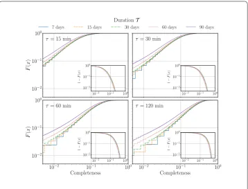
Figure1portrays the cumulative distribution function (CDF) of the completeness of 1.8 million trajectories from our reference dataset when different combinations ofT andτ

Figure 1CDF of completeness. Cumulative distributions of the completeness of trajectories over 1.8 million users for different combinations of the observing durationTand the temporal resolutionτ

• Seamless trajectories with completeness equal to1are extremely rare in mobile phone data, under any combination ofT andτ. Even with short observation periods (T = 7 days) and low resolution (τ= 2hours), not a single complete trajectory is extracted from our reference dataset, despite the large user population. In fact, less than1%of users would satisfy a minimum completeness requirement of0.5, which allows half of the locations to be unknown; and, more than20%of trajectories do not even meet the degree of completeness0.1,i.e., miss9locations out of10. The fact that such poor figures refer to the best case,i.e., the less demanding combination ofT andτ, illustrates well the severity of the sparsity problem in CDR datasets.

• The duration of the observation period has a marginal impact on trajectory

completeness. More precisely, and as one would expect, slightly higher completeness is recorded for trajectories that span a shorter observation period whenT ∈[30, 90] days; however, and quite interestingly, completeness hardly varies whenT ≤30days. We argue that the result can be linked to the weekly periodicity of human activities (which entail a reduced difference forT ∈[7, 30]days), plus seasonal effects such as summer holidays that only intervene over long timescales (T ≥30days in our dataset).

• The temporal resolution has a stronger effect on completeness. For instance, when

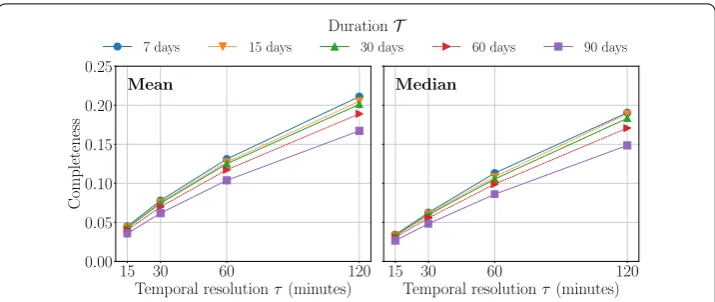
T = 30days, only8%of the trajectories have completeness above0.1whenτ= 15 minutes, whereas the same percentage grows to26%,53%and75%whenτ= 30,60 and120minutes, respectively. To better understand the scaling of completeness with the temporal resolution, we show in Fig.2the mean and median values of

Figure 2Completeness versus temporal resolution. The left and right plots show the mean and median of the completeness of trajectories, respectively, as the function of temporal resolutionτ

grows almost linearly (Pearson correlation coefficients are at0.981and0.983, for the mean and median, respectively) withτ in the range15to120minutes, under all observation periodsT. The takeaway message is that one cannot easily escape the tradeoff that higher temporal resolution incurs into curbed completeness in CDR data. Overall, our results highlight that the vast majority of trajectories from a typical CDR dataset only capture a rather small portion of the complete user mobility. Based on Fig.2, we quantify the fraction of known positions between 5% and 20% on average, depending on the temporal resolution needed for the analysis. These results are well aligned with the outcome of user filtering in previous studies that leverage mobile phone data, where only a small subset of users displays sufficient completeness and is retained for analysis [3,4, 19].

3.2 A statistical model of completeness

As a further contribution to the characterization of the sparsity problem, we derive a data-driven model of CDR-based trajectory completeness. The model can be leveraged to ob-tain a quick, approximate estimate of the completeness of trajectories extracted from a CDR dataset, by merely providing the timespan of the CDR data and the desired temporal resolution.

In order to derive the model, we fit theoretical distributions to the completeness proba-bility density function (PDF) and link the distribution variables to the system parameters

T andτ. Earlier studies have shown that mobile communication activity tends to follow long-tailed distributions across users [20]. Since the usage patterns of mobile devices di-rectly determine completeness, it makes sense to look at heavy-tailed theoretical distribu-tions. We run a maximum likelihood estimation of the variables of six standard long-tailed distributions (Generalized Pareto, Lévy, Power-law, Lognormal, Gamma, and Weibull) on the empirical PDF of completeness. We then evaluate the quality of fitting via the coef-ficient of determinationR2_{, and by running the Kolmogorov-Smirnov test to obtain the} DKSstatistic.

Table 2 Empirical fittings of the completeness of trajectories. Fitting quality of six standard long-tailed distributions to the empirical PDF of trajectory completeness, in terms ofR2andDKS. Rows refer to different combinations of observation periodT and time resolutionτ. Best-fitR2_and DKSare highlighted in bold

Duration T

Resolution τ

Weibull Lognormal Gamma Pareto Levy Power law

DKS R2 DKS R2 DKS R2 DKS R2 DKS R2 DKS R2

7 d 15 min 0.0334 0.9990 0.03180.9973 0.3710 0.4679 0.0495 0.9969 0.2509 0.8046 0.3538 0.5031 30 min 0.0302 0.99930.0345 0.9967 0.0548 0.9962 0.1716 0.8973 0.2649 0.7848 0.3587 0.4894 60 min 0.0278 0.99900.0372 0.9958 0.0475 0.9977 0.1198 0.9516 0.2888 0.7506 0.4162 0.2041 120 min 0.0375 0.99720.0443 0.9938 0.0629 0.9853 0.1043 0.9768 0.3238 0.6977 0.2456 0.7450

15 d 15 min 0.0264 0.9986 0.02330.9984 0.3594 0.5007 0.0627 0.9893 0.2620 0.7853 0.3949 0.4120 30 min 0.0208 0.99950.0264 0.9980 0.0271 0.9991 0.0724 0.9851 0.2765 0.7647 0.3576 0.4975 60 min 0.0188 0.99970.0279 0.9974 0.0257 0.9987 0.0935 0.9719 0.2997 0.7315 0.3176 0.6076 120 min 0.0254 0.99870.0332 0.9961 0.0913 0.9572 0.1880 0.8780 0.3349 0.6792 0.2721 0.7116

30 d 15 min 0.0239 0.9985 0.0207 0.99850.3514 0.5261 0.0700 0.9835 0.2619 0.7872 0.3829 0.4365 30 min 0.0205 0.99920.0216 0.9983 0.02030.9991 0.1528 0.8976 0.2763 0.7661 0.3912 0.4149 60 min 0.0149 0.99960.0263 0.9975 0.0289 0.9982 0.0895 0.9702 0.3003 0.7346 0.3131 0.6212 120 min 0.0239 0.99840.0315 0.9962 0.0995 0.9479 0.1069 0.9538 0.3337 0.6893 0.3154 0.6176

60 d 15 min 0.0266 0.9980 0.02390.9977 0.1990 0.8284 0.0458 0.9934 0.2527 0.8076 0.3850 0.4156 30 min 0.0233 0.99850.0234 0.9976 0.0286 0.9974 0.1944 0.8669 0.2649 0.7903 0.3897 0.4212 60 min 0.0207 0.99850.0264 0.9970 0.0310 0.9980 0.0772 0.9769 0.2883 0.7622 0.3451 0.5635 120 min 0.0245 0.99750.0316 0.9958 0.0754 0.9750 0.0946 0.9617 0.3209 0.7196 0.3491 0.5070

90 d 15 min 0.0298 0.99540.0329 0.99540.3619 0.5248 0.0322 0.9954 0.2371 0.8390 0.3866 0.4528 30 min 0.0336 0.9958 0.03350.9950 0.0583 0.9864 0.0398 0.9942 0.2487 0.8264 0.3819 0.4774 60 min 0.0305 0.99600.0355 0.9944 0.0454 0.9913 0.0611 0.9843 0.2705 0.8020 0.3231 0.6123 120 min 0.0369 0.99400.0379 0.9932 0.0486 0.9927 0.0760 0.9743 0.2998 0.7687 0.3359 0.5885

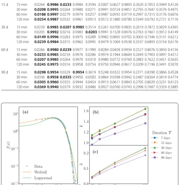
Figure 3Fitting completeness into long-tailed distributions. (a) Empirical PDF of the completeness of 1.8 million user trajectories, with Weibull and lognormal theoretical fittings, forT = 60 days andτ= 60 minutes. (b)(c) Weibull variableskandλversus the temporal resolutionτand observation periodT

Fig.3(a). The Weibull distribution emerges as a clear winner, as it prevails in 32 out of 40 cases in Table2.

The PDF of the Weibull distribution is expressed asfWeibull(x) =kλ(

x

λ)

k–1_e–(x/λ)k

parameter,τ. Also, the observation timeT introduces an offset to the linear relationship. We thus modelkˆ= [τ ×(4.569 – 0.01037T) + 1086.5 – 1.14515T]×10–3 _andλˆ_{= [τ×} (1.814 – 0.00379T) + 26.23 – 0.07659T]×10–3_{, and the CDF of CDR-based trajectory} completeness asfWeibull(x;k,ˆ λˆ).

4 Missing location inference

In this section, we formalize the problem of trajectory reconstruction from sparse and irregular sampling and discuss how popular features of human mobility can be leveraged to design a sensible solution to the problem.

4.1 Trajectory reconstruction problem

Let us consider mobile phone data spanning an observation periodT. User trajectories are inferred by discretizingT into intervals of durationτ, henceT ={1, . . . ,N}can be re-garded as the set of all time intervals. The actual (i.e., ground-truth) trajectory of a generic individual in the dataset is denoted byL_T ={li|i∈T}, where liis therepresentative lo-cationof the user during theith time slot. When a single mobile communication event is associated to a time intervali, the representative location limaps to the geographic lo-cation associated with the event. This is the geographical position of the antenna that is the most representative of the user location. Although our discussion is general and can accommodate any definition of antenna representativeness, we opt for a strategy of se-lecting the antenna that handles the most communications during the target time sloti. We remark that this approach allows mitigating the so-called “ping-pong” (also referred to as “flickering” or “oscillation”) effect that affects mobile phone data. This phenomenon consists in the mobile device association bouncing across nearby antennas, so that the lo-cation proxy for a same user changes even in absence of physical movement. The effect occurs at fast timescales of seconds [21,22], hence oscillations are highly likely to occur within a single time sloti, which spans tens of minutes or more in our case. In each slot, oscillations are then canceled by the antenna selection process above.

As discussed in Sect.3, trajectories extracted from mobile phone data are usually incom-plete,i.e., no event is recorded during many time intervals, and li=∅for a large fraction ofi’s. LetΩ={i∈T |li=∅}be the set of time instant for which we have location infor-mation for the considered user. We define theobserved trajectoryof non-null locations as LΩ ={li|i∈Ω}; this is the user mobility information that can be derived from the mobile phone data. Let us also denote byΩC=T –Ω the time slots set during which the user location is unknown.

The trajectory reconstruction problem is then that of inferring, based on the sole knowl-edge ofLΩ, an estimated complete trajectoryLˆT ={ˆli=∅ |i∈Ω∪ΩC}such that

arg min

ˆ

L_T 1

|T|

N

i=1

li–ˆli, (1)

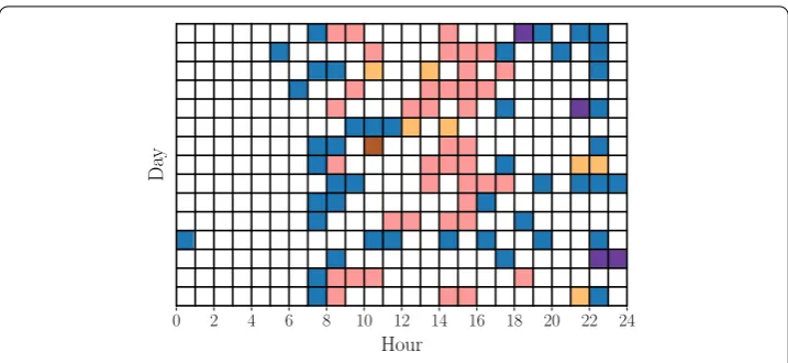
Figure 4Example of the observed trajectory of a user. The trajectory is recored duringT= 15 days and has a degree of completeness in 0.27. Each grid element maps to the representative location associated to each time interval ofτ= 1 hour. Colors map to different places: the most active daytime and nighttime locations are marked in pink and blue respectively; white blocks are missing locations. Figure best viewed in colors

4.2 Design rationale

In order to solve the problem in (1), we have to rely on the known locations of a user,LΩ,

to infer those missing. Several well-known properties of human mobility play in our favor and can be leveraged to solve the problem effectively, as follows.

• Prevalence of static phases.People tend to spend a substantial amount of their time at a few fixed locations (e.g., workplace, school, shopping mall, sports center), where they linger for long continuous periods in the order of hours. Transitions among these locations are instead fairly rapid: in fact, people typically perceive movement phases between points of actual interest as a waste of time and strive to reduce them to a minimum. This results in a pattern of long static phases with fast movements in between [18]. The prevalence of static behaviors allows adopting temporal resolutions that are granular enough to capture the important stay points of each individual, yet are still tractable for reconstruction. For instance, in the example of Fig.4, the user tends to stay for long times at the same location during working hours, and consideringτ= 1hour as done in the plot does not lose substantial positioning information during such hours.

• Overnight invariance.A user is typically at the same location,i.e., at home, during nighttime, as also demonstrated by the fact that even sparse CDR data can be effectively employed to identify dwelling units [14,23]. The observation that most nighttime locations match is important for trajectory reconstruction since mobile phone events tend to be especially scarce overnight, yet knowledge gaps can be filled with a limited amount of observed data during night hours. As an illustrative example, the user in Fig.4is always found at the same place early in the morning, late in the evening, and once overnight: it is apparent that such a location can be sensibly extended to all night hours, which are otherwise very poorly sampled.

• Regularity of movement.Human mobility is strongly regular, from multiple

considered jointly, these results have critical implications for trajectory

reconstruction: they suggest that sparse location data may still be highly informative of the mobility of one individual if such data are sufficiently distributed in time to capture diverse moments of the day and week. This is typically the case for mobile phone data, which feature a combination of temporal irregularity of the sampling and long observation periodsT. As an example, in the case of Fig.4, the fact that the user generates CDR events at different moments of the morning, working hours, and evening allows depicting a fairly complete picture of her mobility pattern during a typical day, by observing mobile communication samples for a sufficiently long amount of time (15 days in the considered sample).

5 Context-enhanced trajectory reconstruction

Context-enhanced Trajectory Reconstruction (CTR) is a novel trajectory reconstruction approach that solves the problem in (1), by receiving the observed trajectoryLΩ as the

input, and generating an estimated complete trajectoryLˆT. To this end,CTRbuilds upon the observations in Sect.4.2, via the three steps detailed next. The notation employed throughout the discussion is summarized in the Abbreviations section.

5.1 Nighttime trajectory reconstruction

The first step inCTRaims at reconstructing missing portions of a trajectory during the night hours. The rationale is that, as seen in Sect.4.2, these are easily reconstructed from the extractable knowledge about users’ home locations, which is also straightforward to derive from mobile phone data. Specifically, we assume that nighttime spans between 10 PM and 9 AM of the subsequent day: this period is adapted to the typical schedule in the Latin America country where our data is collected, but are easily adjusted to any other settings with statistical data on the local population habits. For each user in the dataset, we proceed as follows.

We first identify the most frequent location visited by the user during nighttime, which we nameˆlH. Then, we verify thatˆlHaccounts for a conservative 80%(or more) of the po-sitions of the user during the night period. If this is not the case, we deem that the result is not consistent enough to establish with high confidence the actual home location of the user, and we skip the nighttime trajectory reconstruction step. Otherwise, we identifyˆlH as the home location of the user. When applied to our reference dataset of 1.8 million sub-scribers, this strategy allowed assigning a home location to 0.72 million users, equivalent to 42% of the whole population.

If a home locationˆlHis identified, each 10 PM–9 AM period is processed separately for every day. The user is considered to be at home only in periods where no location other thanˆlHis observed in the data: in this case, all time intervalsiin the period are added to a setΩH. Otherwise, if at least one location different fromˆl_His present during a 10 PM–9 AM period, we consider that the user may not have spent that specific night at home, and no modification is made toΩH. Once all days have been processed, we assign the home location to all slots inΩH_,i.e.,ˆ_l

i=ˆlH,∀i∈ΩH. We then update the known trajectory as

ˆ

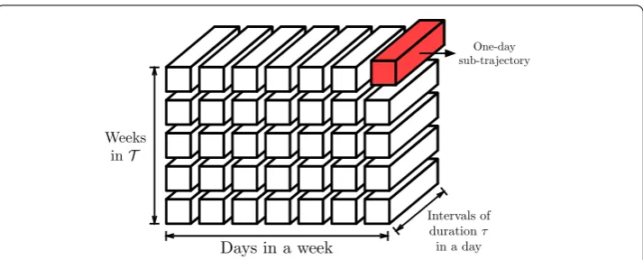
Figure 5Example of the location tensor of a userX. A trajectoryL_T is represented as daily and weekly combinations of one-day sub-trajectories

5.2 Seamless trajectory reconstruction with tensor factorization

The second step ofCTRaims at reconstructing the trajectory during the remaining time intervals inΩC, by tailoring state-of-the-arttensor factorizationtechniques to our prob-lem. Tensor factorization exploits redundancy to recover missing data; in our context, redundancy is created by the regularity of human movement, which creates repeated pat-terns of visited locations over the many days and weeks covered by a CDR dataset, as discussed in Sect.4.2.

We start by organizing the trajectory data of a user into a three-dimensional ten-sor format, as illustrated in Fig. 5. The location tensor X has dimensions that reflect the weekly, daily, and instantaneous (with granularityτ) mobility of the user. Therefore

X ∈RNw×Nd×2Nτ_{, whereN}

wis the number of weeks in the observation period,Ndis the number of days in a week, andNτ is the number of time slots in a day.

A trajectoryL_T is transformed intoXvia the following two steps:

• First, the trajectory is split into multiple one-day sub-trajectories. Each one-day sub-trajectory is then converted into a one-dimensional vector: for instance, the sub-trajectory of thejth_{day of theith week is denoted byx}

i,jand satisfies

xi,j= (l(x)ni,j,1, l (y) ni,j,1, . . . , l

(x) ni,j,Nτ, l

(y) ni,j,Nτ)∈R

2Nτ_{, wherel}(x) k andl

(y)

k are the two coordinates that identify the location at time stepk, forlk= (l(x)k , l

(y) k ).

• Second, we enter all of the one-day sub-trajectories of a user trajectory into the location tensor by organizing them into a matrix of one-day sub-trajectories for allNw weeks in the observation periodT,i.e.,X= [xi,j]Nw×Nd={Xi,j,k}Nw×Nd×2Nτ.

The location tensor X is partially filled with the original incomplete trajectory from mobile phone data, as well as with the inferred overnight locations as per Sect.5.1. At this stage, the location tensor includes information for time slots inΩ∪ΩH. However, the tensor is still relatively sparse, as the setΩCof time intervals where locations are missing is still large. In our reference dataset, the location tensors have an average density of 0.63 (where 1 denotes a complete tensor) when first generated.

decompo-sition (CPD) [27] of the tensorX ∈RNw×Nd×2Nτ _{into threeR-rank matrices A}∈RNw×R_,

B∈RNd×R_{, and C}∈R2Nτ×R_{, where each value}X

i,j,k in the tensor is approximated as

Xi,j,k= R

δ=1Ai,δBj,δCk,δ. In our experiments, we set the rankRto the minimum

cardinal-ity of the tensor dimensions,i.e.,R=min(Nw,Nd, 2Nτ). This value entails a small number

of hyperparameters in tensor decomposition, and is well within the upper bound of the tensor rankmin(NwNd, 2NwNτ, 2NdNτ), which cannot be otherwise computed with a

fi-nite algorithm [27]. For simplicity, we employ the concise notationJA, B, CKfor the CPD using matrices A, B and C. The TF problem is then

ˆ

A,Bˆ,Cˆ =arg min

A,B,C

(i,j,k)∈Ω∪ΩH

Xi,j,k–JA, B, CKi,j,k 2

+λA2_F+B2_F+C2_F, (2)

whereλis a penalty parameter to avoid overfitting [27] and · F is the Frobenius norm. The solution to the problem in (2) is an estimation of the complete tensorXˆ=JAˆ,Bˆ,CˆK, which thus recovers the missing locations inΩC. In other words, we are seeking a ten-sor that hasR-rank CPD decomposition and that fits the observed locations as closely as possible.

In fact, (2) is a standard TF problem, which does not account for contextual specificities that can improve the solution. Specifically, the formulation in (2) treats each dimension and every single value of the tensor equally, while human mobility patterns exhibit non-uniform importance of dimensions and values. Indeed, (i) daily periodicities tend to be stronger than weekly ones [3], and (ii) consecutive time slots, hence nearby values in a same one-day sub-trajectory vector, show a strong correlation in terms of locations of the user [18]. In the light of these considerations, we customize the TF problem for location inference, by introducing two additional elements to the optimization problem in (2).

The first element emphasizes daily repetitive mobility patterns by means of Toeplitz matrices. Toeplitz matrices allow modelling relationships between specific elements in the location tensor. For instance, given a matrix P = [pi,j]N×N and a Toeplitz matrix

Q= Toeplitz(1, –1, 0)N×N, then the productPQ2F represents the sum of the differences

between consecutive values in the original matrix P,i.e., expands toN_i=1N_j=0(pi–1,j– pi,j)2F. Therefore, we construct a matrix D = Toeplitz(1, –1, 0)Nd×Ndas illustrated in Fig.6;

then, the expressionX×dD2F, where×dis thetensor-matrixproduct [27] such that (X×dD)i,m,k=

Nd

n=1Xi,n,kDm,n, represents the sum of squared differences of location co-ordinates at the same hour of consecutive days. In our case,X is decomposed via CPD

intoJA, B, CK, hence we have

JA, B, CK×dD i,m,k= Nd n=1 R δ=1

Ai,δBn,δCk,δDm,n

= R

δ=1

Ai,δ

_N d

n=1

Dm,nBn,δ

Ck,δ

= R

δ=1

Ai,δ(DB)m,δCk,δ (3)

and equivalently,JA, B, CK×dD=JA, DB, CK. MinimizingJA, DB, CK2Fimplies reduc-ing the diversity of locations at a same hour across individual days.

A similar approach is then adopted to ensure that the solution to the TF problem favors the similarity of locations in consecutive time intervals. Here, we construct a Toeplitz ma-trix T = Toeplitz(1, 0, –1, 0)2Nτ×2Nτ, and denote by×τ the tensor-matrix product such that

(X×τD)i,m,k= 2Nτ

n=1Xi,m,nTk,n. Recall that each daily sub-trajectory is a one-dimensional vector (l(x)₁ , l(y)₁ , l(x)₂ , l(y)₂ , . . . )∈R2Nτ_{, hence the x-axis (respectively, y-axis) of two}

consecu-tive locations are separated by a coordinate of the other type. Then, including in the min-imization problem the termX×τT2_F=JA, B, TCK2_Fallows constraining the diversity

of locations between consecutive hours in a same day.

Embedding both elements above in (2) leads to an enhanced TF problem

arg min

A,B,C

(i,j,k)∈Ω∪ΩH

Xi,j,k–JA, B, CKi,j,k 2

+λA2_F+B2_F+C2_F

+λdJA, DB, CK 2

F+λτJA, B, TCK 2

F (4)

whereλdandλτ weight the importance of similarity across time slots that are 24-hour

apart and adjacent, respectively. The problem in (4) is a combination of multiple least square problems, and is efficiently solved by means of an alternating least square (ALS) technique [27].

The complete tensor estimationXˆcontains the original locations of the user extracted from the mobile phone data during time instants inΩ, the locations inferred during night hours inΩHas per Sect.5.1, and those estimated by solving (4) for all time slots inΩC. Therefore,Xˆcan be used to fill an updated trajectoryLˆ_T ={li|i∈Ω}∪{ˆli|i∈ΩH∪ΩC}, which isseamless,i.e., covers the whole observation periodT.

5.3 Homogeneous quantization of locations

The locations in the original mobile phone data, as well as those inferred for night hours, match the position of cellular network towers. Instead, the solution of the enhanced TF problem in (4) returns locations whose coordinates are real values, which may not match the position of actual cellular towers. Since it is desirable that the reconstructed trajectory has consistent properties (including a homogeneous quantization of the locations that is based on the cellular infrastructure deployment), the third step inCTRaims at associating each location estimated as per Sect.5.2to the position of a real-world cellular tower.

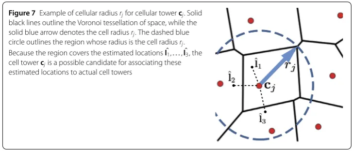
Figure 7Example of cellular radiusrjfor cellular towercj. Solid black lines outline the Voronoi tessellation of space, while the solid blue arrow denotes the cell radiusrj. The dashed blue circle outlines the region whose radius is the cell radiusrj. Because the region covers the estimated locationslˆ1,. . .,lˆ3, the

cell towercjis a possible candidate for associating these estimated locations to actual cell towers

i∈ΩCby one of the cell tower positions cj∈C. To this end, we first design a sensible cost function for determining the suitability of a match (ˆli, cj) between a generic location and a cell tower position. The cost function, denoted byf(ˆli, cj), accounts for (i) the geographic distance betweenˆliand cj, and (ii) the popularity of the tower cj, as:

f(ˆli, cj) = ⎧ ⎨ ⎩

1/ej ifcj,ˆli ≤rj,

+∞ otherwise. (5)

In expression (6) above:ejis the number of communication events that are generated by all the users in the dataset and associated to the cellular tower cjin the mobile phone data;

· denotes the geographic distance between the two location parameters; and,rjis the cellular radiusof tower cj,i.e., the maximum distance between the actual tower position

cjand the farthest corner of its Voronoi tessellation cell [28] as illustrated in Fig.7. The cell tower replacing an estimated locationˆliis that satisfying

arg min

cj∈C

f(ˆli, cj). (6)

In other words, minimizing the cost function limits the selection of matching cell towers for an estimated locationˆlito those within distancerjofˆli; then, it picks the candidate having the highest probability of occurrence in the data, hence adopting a wisdom-of-the-crowd approach that has already proven effective in personal mobility analysis [29].

6 Validation

In order to validate the proposedCTRsolution, we employ a set of ground-truth trajecto-ries with completeness equal to 1, presented in Sect.6.1. We generate incomplete trajec-tories from the ground-truth data, following the same sampling process observed in our reference CDR dataset, as described in Sect.6.2. Then, complete trajectories are recon-structed withCTRfrom the downsampled ones, and compared against the ground-truth, in Sect.6.3: the level of agreement lets us comment on the quality of the reconstruction.

6.1 Fine-grained ground-truth trajectories

from Internet access rather than voice calls, they entail a sensibly higher frequency in location sampling. When considered jointly with CDR, rich mobile Internet data allows obtaining the complete trajectories of 1450 users over an observation periodT of two consecutive weeks, and with a temporal resolution ofτ = 1 hour. If multiple samples are recorded in the same time slot, the unique location is determined as that of the cell tower which most events are associated with. In other words, we have 1450 complete trajectories having observation setsΩ=T. In each of them, all the locations are known,i.e.,LΩ={li| i∈Ω}=LT. We remark that the available fine-grained ground-truth trajectories bound our validation to a two-week period. We leave to future analyses, based on mobility data covering longer periods, the assessment of the impact of the trajectory duration on the accuracy of the completion process.

6.2 Incomplete trajectories

Incomplete trajectories are generated by downsampling the ground-truth ones. For in-stance, a trajectory with completeness 0.3 is derived from a two-week ground-truth tra-jectory having 14×24 = 336 time slots by keeping the locations in 101 time slots and dis-carding the rest. Here, the sampling process must be chosen appropriately: for instance, a uniform random selection would result in a temporal distribution of retained locations that is inconsistent with that produced by mobile communication events in CDR. We en-sure that the incomplete trajectories mimic the temporal sampling properties of those extracted from CDR as follows: (i) we construct an empirical distribution of the probabil-ity that events are recorded at each time slots, based on CDR data of all 1.8 million users in our dataset; (ii) we set the desired completeness valuekthat shall characterize the out-put incomplete trajectory; (iii) we retain a fractionk of the overall location samples in one complete trajectory according to a random selection of time slots that follows the empirical distribution above. Performing this approach once leads to an artificial missing setΩC, and results in a down-sampled incomplete trajectoryLΩ={li|i∈Ω}(recall that Ω=T –ΩC).

This approach lets us produce a large amount of downsampled trajectories out of the 1450 ground-truth ones, and gives us enough flexibility to carry out a comprehensive val-idation. Specifically, we generate 3×105_{incomplete trajectories with completeness} rang-ing from 0.01 to 0.5, which allows testrang-ingCTRtrajectory reconstructions in a wide diversity of settings.

6.3 Quality ofCTRtrajectory reconstruction

We runCTRon the incomplete CDR-like data and update the incomplete CDR-like tra-jectories asLˆT ={li|i∈Ω} ∪ {ˆli|i∈ΩC}. We then assess the quality of the reconstructed trajectoriesLˆ_T against the complete ground-truth known locationsL_T.

The performance metric we adopt iscell displacement, which expresses the MAE used in (1) in terms of mobile network cells, as

(LˆT,LT) = 1

|L_T|–|LΩ|

i∈T\Ω

li,ˆli rj

. (7)

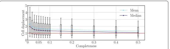
Figure 8Performance ofCTRin cell displacement. Cell displacement of locations inferred viaCTRwith respect to the actual ones, versus the completeness of the original trajectory. Candlesticks highlight the mean (light blue), median (dark blue), 25th_{and 75}th_{percentiles (box), and 10}th_{and 90}th_{percentiles (errorbars). The}

horizontal line (red) highlights a one-cell displacement

for which li= cj. Expression (7) implies that the cell displacement is computed only based on locations that are missing in the original data (i.e., for time instants inT \Ω), and known user positions do not affect it. Unlike MAE, cell displacement compensates for the very diverse density (hence radius) that cellular towers tend to have in different regions of a large geographic area and provides a relative measure that is comparable across all locations.

The validation results are summarized in Fig.8, where the cell displacement measured in the trajectories reconstructed byCTRis shown against the completeness of the input CDR-like data. The candlesticks report the mean and median cell displacement, as well as the 10th, 25th, 75th, and 90thpercentiles. The horizontal red line highlights a cell dis-placement of 1: below this value, the estimation error is lower than spatial precision of the original mobile phone data,i.e., the geographical coverage radius of the cell tower the user is presently associated to. Therefore, the error of the completion process is smaller than that inherent to the original data.

The most important remark is that the median cell displacement is always between 1 and 2, which denotes a substantial accuracy in the reconstructed trajectories: even under completeness levels as low as 1%, estimated locations are typically placed in a cell that is immediately adjacent to the correct one, or one cell further. More complete original trajec-tories provideCTRwith added information to fill gaps in the data, leading to an improved performance where the typical estimation error is pushed closer to the correct cell. Inter-estingly, the gain of accuracy is higher at low completeness levels, and a trajectory with just 5%completeness already reduces the median cell displacement to less than 1.5. Some variability is observed around the median, which is however natural, given the hetero-geneity that characterizes the mobility patterns and communication activities of different users.

7 Revisiting key results in the literature

As mentioned in Sect.1, mobile phone data are the cornerstone of many seminal works on large-scale human mobility analysis. All such works (i) employ raw CDR datasets that are highly incomplete, and (ii) possibly adopt substantial user filtering. However, if and how trajectory incompleteness and user filtering effect—and possibly bias—the outcome of these studies is unclear. Our aim in this section is shedding light on this matter, which also lets us demonstrate the importance of trajectory reconstruction in mobile phone data analysis.

To this end, we runCTRon the reference dataset presented in Sect.3and reconstruct all trajectories which have completeness higher than 1%in the original data. Selecting such a lower threshold on completeness bounds the typical cell displacement to a small value according to the validation in Sect.6, hence ensure high confidence in the quality of the estimated locations; moreover, a 1%completeness threshold allows retaining 95%of the user population. Overall, we reconstruct the complete trajectories of around 1.7 million individuals in a large geographic region, with a temporal resolution ofτ = 1 hour during three months.

We then reproduce three key studies on human mobility, using both the original CDR dataset and the complete trajectory data returned byCTR, and discuss the eventual differ-ences that we observe in the results. The three analyses are separately presented next.

7.1 Laws of individual mobility

In an important study appeared in Nature in 2008, Gonzalezet al.[3] derive a seminal model of individual human mobility based on CDR data. The data-driven analysis reveals that the travel distances of single users between two consecutive locations follow a trun-cated power-law. Formally, for any given individual, her travel distancerbetween two consecutive events follows a truncated power-lawP(r|rg)∼rg–αF(r/rg), wherergis the radius of gyration,a_{andF(x) is a function such thatF(x)∼x}–α_{forx< 1 andF(x) rapidly}

decreases for x> 1. This expression indicates that human movements resemble aLévy flightthat follows a power-lawP(r)∼r–α_{within a geographical region bounded byr}

g; long displacements beyond such region are instead increasingly rare.

These key insights are obtained from a random sample of 1.67%of the total 6 million users, and the trajectories of the selected users are largely incomplete, with less than one location per user and per day recorded on average. We run the same analysis on the seam-less trajectories of 1.7 million users, and show in Fig.9how considering complete move-ment data of a full user population affects the results. Clearly, we look now at a complete set of events—one per time slot—and the travel distanceris computed between the lo-cations in any two subsequent time slots. This ultimately results in a more comprehensive view of individual travel distances. We make the following considerations.

• As a preliminary result in their analysis, Gonzalezet al.find that the travel distances and radiuses of gyration aggregated over the whole user population follow truncated power laws(x+x0)–βe–x/k. We confirm that this is also the case under complete trajectory data, as shown in the top plots of Fig.9. The exponent values are also consistent, as Gonzalezet al.findβr = 1.77andβrg= 1.65, whereasβr= 1.78and βrg= 1.68from our complete trajectory data. However, we remark a sensible

Figure 9Revisited results from [3]. Distributions of travel distancer, radius of gyrationrg, and conditional travel distancer(with respect tor/rg) for original and complete trajectories

(i.e., incomplete) CDR-based trajectories but is reduced in the complete data, where the cutoff occurs instead at 175 km. We ascribe the difference to the fact that completion often leads to add missing locations that are far from the linear interpolation between CDR positions, such as those generated by infrequent but recurrent long-haul trips. Our conclusion is that, CDR data sparsity risks to both underestimate long trips, and overestimate the region within which the Lévy flight behavior of human mobility occurs.

• Concerning individual movements, we can reproduce the truncated power-law behavior found by Gonzalezet al.with both our sparse CDR-based trajectories and the complete ones reconstructed viaCTR. This is illustrated in the bottom plots of Fig.9. In the original work, the authors find an exponentα≈1.2, and we estimate the

αparameter at1.8and1.4for original and complete trajectories. These exponents are

qualitatively consistent since they all are in the(1, 3)range that characterizes Lévy walks [30].

• We ascribe the quantitative differences with respect to [3] to the inherent specificity of each dataset. Although we also use locations from voice calls as in [3], the data refer to very different cultural and economic settings (i.e., a European country and a South American one) and geographical span (our country covers a territory that is four times wider than the largest country in Europe).

Figure 10 Revisited results from [5]. Ratio of trajectories with uniqueness|U|= 1 for a number of spatiotemporal points in the abscissa, for original (left) and complete (right) trajectories

7.2 Uniqueness of individual trajectories

The work by De Montjoyeet al.[5], published in Scientific Reports in 2013, is the first to raise significant concerns on the privacy of users whose communication activities are recorded in CDR datasets. The study unveils the very highuniquenessof individual trajec-tories: knowing a few random time-stamped locations of an individual allows pinpointing her trajectory within the mobile phone data of a large user population. Notably, the au-thors show that 4 random li’s identify one specific user among 1.5 million individuals 95% of times. In practice, the result implies that an adversary would need minimal knowledge about the mobility of a victim in order to perform a re-identification attack on a CDR dataset. The tests leading to the conclusion above consider a large user population but rely on raw CDR data that is highly incomplete: on average, a user only has approximately 19 unique locations observed in a month from 4200 cell towers.

Figure10depicts how complete trajectories affect the results. The plots show how many trajectories in the dataset are uniquely identified by knowing a random number of time-stamped locations (in the abscissa), with incomplete CDR data, and with seamless recon-structed trajectories. The result with incomplete data is very well aligned with that of De Montjoyeet al.However, the difference with complete trajectories is striking: for the low number of locations considered in [5], the uniqueness is reduced by around one order of magnitude when the location information is seamless. The contrast lets us argue thatthe extremely high uniqueness identified by De Montjoye et al. is mainly caused by the diverse temporal patterns of the mobile communications of each user, rather than by his/her dis-tinctive mobility.In other words, many users tend to have similar complete trajectories, and sampling them randomly yields limited uniqueness; it is instead the sparse sampling of the trajectories inherent to CDR that introduces an artificial temporal diversity and leads to dramatically increased uniqueness.

Figure 11 Revisited results from [4]. Distributions of the entropy and maximum theoretical predictability derived with (i) the incomplete original CDR-based trajectories of 8000 users filtered with the method in [4], (ii) the complete trajectories of all 1.7 million users, and (iii) the complete trajectories of the same 8000 users considered in the first case

7.3 Next-location predictability

The high theoretical predictability of human mobility was first exposed by Songet al.[4], in a famous paper that appeared in Science in 2010. In that work, the authors model the movement of each user as a time series of locations extracted from mobile phone data. They then measure the entropy rate of the probability of finding a particular time-ordered subsequence in the trajectory of the user. Finally, they compute the maximum predictabil-ity of each outcome from the entropy rate, by using Fano’s inequalpredictabil-ity. The analysis con-siders 45,000 users (out of a total population of 10 million) with trajectory completeness higher than 0.2, at least 0.5 calls/hour and more than 2 unique recorded locations during an observation period of 14 weeks. Based on these data, the theoretical predictability is found to have a very high upper bound at around 93%.

We repeat the experiment with our reference dataset and trajectory reconstruction method. We run the filtering adopted by Songet al.on our original CDR data and extract 8000 users: this maps to around 0.44%of the available population, which is very close to the 0.45%considered in [4]. The probability distribution of the maximum predictability across the retained users is labeled asoriginalin Fig.11. The mean predictability is at 81%, which is high yet quite far from the 93%found by Songet al.: As users are selected in the exact same way in the two cases, we ascribe the difference to the diverse mobility habits of the user populations in the two datasets, which are collected in different countries, at different scales, and during different time periods.

More interesting to our study is thus the comparison of the predictability obtained with the incomplete trajectories of 0.44%of the users, and that resulting from the seamless trajectories of the full available population (i.e., 1.7 million users), reconstructed through

larger population lets us account for the vast majority of fairly static users, and reveals that people’s movements are on average even easier to predict than estimated in [4].

In order to verify our hypothesis, we show in Fig.11the predictability distribution for the complete, reconstructed trajectories of the same 8000 users that are retained from the original data by the filtering proposed in [4]. The result, tagged ascomplete/filtered

is very consistent with that derived with the sparse CDR-based trajectories of those sub-scribers,i.e., theoriginalcurve. The result supports our intuition that it is the popula-tion sampling and not the reconstrucpopula-tion process that determines the striking difference in the figure.

8 Conclusions

We have investigated the problem of sparsity in trajectories inferred from mobile phone data. We have quantified the issue in a representative real-world dataset, proposed a novel solution, namedCTR, to reconstruct a seamless trajectory from sparse CDR data, and val-idated our methodology using ground-truth movement patterns. We have also demon-strated the importance of trajectory reconstruction by revisiting well-known results on human mobility based on raw CDR, and showing that complete trajectories can in some cases affect the outcome of those analyses substantially.

Funding

This work was supported by the ERANET CHIST-ERA MACACO and is performed in the context of the EMBRACE Associated Team of Inria and STIC AmSud MOTIF.

Abbreviations

T,observation period of a trajectory;LT={li|i∈T},ground-truth trajectory;Ω={i∈T|li=∅},observed period of a

trajectory;LΩ={li|i∈Ω},observed trajectory;ΩC=T–Ω,unknown period of a trajectory;

ˆ

LT={ˆli=∅ |i∈Ω∪ΩC},estimated trajectory;∅,empty set;li,location of theith time slot.

Availability of data and materials

The datasets we use in this study contain sensitive personal information and are protected by non-disclosure agreements with the data owners, which prevents public disclosure. We understand and appreciate the need for transparency in research, however we cannot share access to confidential datasets used.

Ethics approval and consent to participate

Data collection was approved by the data owners, and written informed consent has been obtained for all study participants.

Competing interests

The authors declare that they have no competing interests.

Authors’ contributions

Designed the study: GC, AV, and MF. Collected and analyzed the data: GC and CS. All authors wrote and approved the final manuscript.

Author details

1_{INRIA, Université Paris-Saclay, Palaiseau, France.}2_{École Polytechnique, Université Paris-Saclay, Palaiseau, France.} 3_{CNR-IEIIT, Torino, Italy.}4_{Grandata Labs, San Francisco, USA.}

Endnote

a _{The radius of gyration is a scalar metric assessing the overall mobility of a user. For a trajectoryL}

T, it is computed as

rg= 1

|T|i∈Tli,lC2, wherelC=_|T1_|i∈Tliis the center of mass of all the locations inLT.

Publisher’s Note

Springer Nature remains neutral with regard to jurisdictional claims in published maps and institutional affiliations.

References

1. Blondel VD, Decuyper A, Krings G (2015) A survey of results on mobile phone datasets analysis. EPJ Data Sci 4(1):10.

https://doi.org/10.1140/epjds/s13688-015-0046-0

2. Naboulsi D, Fiore M, Ribot S, Stanica R (2016) Large-scale mobile traffic analysis: a survey. IEEE Commun Surv Tutor 18(1):124–161.https://doi.org/10.1109/comst.2015.2491361

3. Gonzalez MC, Hidalgo CA, Barabasi A-L (2008) Understanding individual human mobility patterns. Nature 453(7196):779–782.https://doi.org/10.1038/nature06958

4. Song C, Qu Z, Blumm N, Barabasi A-L (2010) Limits of predictability in human mobility. Science 327(5968):1018–1021.

https://doi.org/10.1126/science.1177170

5. de Montjoye Y-A, Hidalgo CA, Verleysen M, Blondel VD (2013) Unique in the crowd: the privacy bounds of human mobility. Sci Rep 3(1):1376.https://doi.org/10.1038/srep01376

6. Ahas R, Silm S, Saluveer E, Järv O (2009) Modelling home and work locations of populations using passive mobile positioning data. In: Gartner G, Rehrl K (eds) Location based services and TeleCartography II: from sensor fusion to context models. Springer, Berlin, pp 301–315.https://doi.org/10.1007/978-3-540-87393-8_18

7. Schneider CM, Belik V, Couronne T, Smoreda Z, Gonzalez MC (2013) Unravelling daily human mobility motifs. J R Soc Interface 10(84):20130246.https://doi.org/10.1098/rsif.2013.0246

8. Ferreira N, Poco J, Vo HT, Freire J, Silva CT (2013) Visual exploration of big spatio-temporal urban data: a study of New York city taxi trips. IEEE Trans Vis Comput Graph 19(12):2149–2158.https://doi.org/10.1109/TVCG.2013.226

9. Zhang D, Zhao J, Zhang F, He T (2015) coMobile: real-time human mobility modeling at urban scale using multi-view learning. In: Proceedings of the 23rd SIGSPATIAL international conference on advances in geographic information systems. SIGSPATIAL ’15. ACM, New York, pp 40:1–40:10.https://doi.org/10.1145/2820783.2820821

10. Zang H, Bolot JC (2007) Mining call and mobility data to improve paging efficiency in cellular networks. In: Proceedings of the 13th annual ACM international conference on mobile computing and networking. MobiCom ’07. ACM, New York, pp 123–134.https://doi.org/10.1145/1287853.1287868

11. Oliveira EMR, Viana AC (2014) From routine to network deployment for data offloading in metropolitan areas. In: 2014 eleventh annual IEEE international conference on sensing, communication, and networking (SECON), pp 126–134.

https://doi.org/10.1109/SAHCN.2014.6990335

12. Frias-Martinez E, Williamson G, Frias-Martinez V (2011) An agent-based model of epidemic spread using human mobility and social network information. In: 2011 IEEE third international conference on privacy, security, risk and trust and 2011 IEEE third international conference on social computing, pp 57–64.

https://doi.org/10.1109/PASSAT/SocialCom.2011.142

13. Chen G, Hoteit S, Viana AC, Fiore M, Sarraute C (2018) Enriching sparse mobility information in call detail records. Comput Commun 122:44–58.https://doi.org/10.1016/j.comcom.2018.03.012

14. Ranjan G, Zang H, Zhang Z-L, Bolot J (2012) Are call detail records biased for sampling human mobility? Mob Comput Commun Rev 16(3):33.https://doi.org/10.1145/2412096.2412101

15. Sarraute C, Blanc P, Burroni J (2014) A study of age and gender seen through mobile phone usage patterns in Mexico. In: 2014 IEEE/ACM international conference on advances in social networks analysis and mining (ASONAM 2014), pp 836–843.https://doi.org/10.1109/ASONAM.2014.6921683

16. Jo H-H, Karsai M, Karikoski J, Kaski K (2012) Spatiotemporal correlations of handset-based service usages. EPJ Data Sci 1(1):1.https://doi.org/10.1140/epjds10

17. Hoteit S, Chen G, Viana A, Fiore M (2016) Filling the gaps: on the completion of sparse call detail records for mobility analysis. In: Proceedings of the eleventh ACM workshop on challenged networks. CHANTS ’16. ACM, New York, pp 45–50.https://doi.org/10.1145/2979683.2979685

18. Ficek M, Kencl L (2012) Inter-call mobility model: a spatio-temporal refinement of call data records using a Gaussian mixture model. In: 2012 proceedings IEEE INFOCOM, pp 469–477.https://doi.org/10.1109/INFCOM.2012.6195786

19. Hoteit S, Secci S, Sobolevsky S, Ratti C, Pujolle G (2014) Estimating human trajectories and hotspots through mobile phone data. Comput Netw 64:296–307.https://doi.org/10.1016/j.comnet.2014.02.011

20. Seshadri M, Machiraju S, Sridharan A, Bolot J, Faloutsos C, Leskove J (2008) Mobile call graphs: beyond power-law and lognormal distributions. In: Proceedings of the 14th ACM SIGKDD international conference on knowledge discovery and data mining. KDD ’08. ACM, New York, pp 596–604.https://doi.org/10.1145/1401890.1401963

21. Iovan C, Olteanu-Raimond A-M, Couronné T, Smoreda Z (2013) Moving and calling: mobile phone data quality measurements and spatiotemporal uncertainty in human mobility studies. In: Vandenbroucke D, Bucher B, Crompvoets J (eds) Geographic information science at the heart of Europe. Springer, Cham, pp 247–265.

https://doi.org/10.1007/978-3-319-00615-4-14

22. Katsikouli P, Fiore M, Furno A, Stanica R (2019) Characterizing and removing oscillations in mobile phone location data. In: IEEE WoWMoM 2019—20th IEEE international symposium on a world of wireless, mobile and multimedia networks, Washington DC, United States.https://hal.inria.fr/hal-02110719

23. Douglass RW, Meyer DA, Ram M, Rideout D, Song D (2015) High resolution population estimates from telecommunications data. EPJ Data Sci 4(1):4.https://doi.org/10.1140/epjds/s13688-015-0040-6

24. Oliveira EMR, Viana AC, Sarraute C, Brea J, Alvarez-Hamelin I (2016) On the regularity of human mobility. Pervasive Mob Comput 33:73–90.https://doi.org/10.1016/j.pmcj.2016.04.005

25. Kong L, Xia M, Liu X-Y, Chen G, Gu Y, Wu M-Y, Liu X (2014) Data loss and reconstruction in wireless sensor networks. IEEE Trans Parallel Distrib Syst 25(11):2818–2828.https://doi.org/10.1109/tpds.2013.269

26. Karatzoglou A, Amatriain X, Baltrunas L, Oliver N (2010) Multiverse recommendation: N-dimensional tensor factorization for context-aware collaborative filtering. In: Proceedings of the fourth ACM conference on recommender systems. RecSys ’10. ACM, New York, pp 79–86.https://doi.org/10.1145/1864708.1864727

27. Kolda TG, Bader BW (2009) Tensor decompositions and applications. SIAM Rev 51(3):455–500.

https://doi.org/10.1137/07070111x

28. Portela JN, Alencar MS (2006) Cellular network as a multiplicatively weighted Voronoi diagram. In: CCNC 2006. 2006 3rd IEEE consumer communications and networking conference, 2006, vol 2, pp 913–917.

29. Jeong J, Leconte M, Proutiere A (2016) Cluster-aided mobility predictions. In: Proceedings of the 35th annual IEEE international conference on computer communications. INFOCOM’16.

https://doi.org/10.1109/INFOCOM.2016.7524491

30. Shlesinger MF, Zaslavsky GM, Frisch U (1995) Lévy flights and related topics in physics. Lecture notes in physics, vol 450. Springer, Berlin.https://doi.org/10.1007/3-540-59222-9

31. Paul U, Subramanian AP, Buddhikot MM, Das SR (2011) Understanding traffic dynamics in cellular data networks. In: 2011 proceedings IEEE INFOCOM, pp 882–890.https://doi.org/10.1109/INFCOM.2011.5935313

32. Couronné T, Smoreda Z, Raimond AO (2013) Chatty Mobiles: individual mobility and communication patterns. CoRR abs/1301.6553.http://arxiv.org/abs/1301.6553

33. Hess A, Marsh I, Gillblad D (2015) Exploring communication and mobility behavior of 3G network users and its temporal consistency. In: 2015 IEEE international conference on communications (ICC), pp 5916–5921.