Household CO2-efficient energy management

R E S E A R C H

Open Access

Household CO

₂

-efficient energy

management

Laura Fiorini

and Marco Aiello

FromThe 7th DACH+ Conference on Energy Informatics Oldenburg, Germany. 11-12 October 2018

*Correspondence:[email protected] 1_{Department of Distributed}

Systems, University of Groningen, Nijenborgh 9, 9747 AG Groningen, The Netherlands

Full list of author information is available at the end of the article

Abstract

Residential and commercial buildings are responsible for one third of the total (CO2) emissions in the European Union, which are the main cause of global warming. Although the thermal load has long been considered the primary reason of domestic energy consumptions, the increasing demand for electricity has a non-negligible environmental impact, given that about 40% of electricity is generated by burning fossil fuels. Moreover, the amount of CO2emitted to produce one kWh can greatly vary in time, depending on the sources used to generate it. For instance, the German electricity emissions intensity factor varied in 2017 between 113 and 533 gCO2eq/kWh. This paper proposes a novel CO2-efficient energy management approach to schedule household appliances while minimizing carbon dioxide emissions, given the possibility to change energy carriers (i.e., natural gas and electricity) and to shift loads in time. Several common loads are considered, and their operation is scheduled according to the emission factor of the German power grid. The results show that switching energy carriers can successfully enable up to 40% emissions reductions while indicating that shifting loads in time has little impact.

Keywords: Carbon emissions, Optimal scheduling, Hybrid appliances

Introduction

Climate change is one of the major challenges that the planet is facing, due to the increas-ing emission of (GHG), main responsible for the greenhouse effect. Among these gases, CO2contributes for the largest share, and it is mainly caused by human activities (Stocker et al. 2014). The energy sector is responsible of roughly two-thirds of all GHG emis-sions (OECD2015); in Europe, residential and commercial buildings cause 36% of CO2 emissions (European Commission). Traditionally, Heating Ventilation and Air Condi-tioning (HVAC) demand have been considered the main reasons for domestic energy consumption, and, hence, for CO2emissions (Haines et al.2010). However, the increas-ing ownership of appliances and their use have caused a significant rise in households’ need for electricity (Haines et al.2010), whose environmental impact varies according to the production sources. When using electricity bought from the grid, the amount of CO2 emitted to generate a kWh is determined by the current generation mix. For instance, given a certain amount of power to be produced, the emission intensity factor associated

with a kWh at windy or sunny day is likely to be significantly lower than in a windless and cloudy one, when almost all the power is generated by plants burning fossil fuels.

Demand-side management (DSM) programs aim to control the residential electric use in response to price signals or incentive payments. In a price-based scheme, the con-sumers are offered time-varying rates to modify their demand over time, e.g., to shift the consumptions towards off-peak times; in an incentive-based one, rewards are given to those users who accept to reduce their consumptions when requested by the utility (Siano

2014). The main drivers for DSM programs are the risk of congestions along lines and the possibility to postpone expensive investments costs for the expansion of the infras-tructure capacity, while giving the consumers the chance to reduce their energy bills. By an environmental point of view, while reducing the consumptions has certainly a posi-tive effect, a price-based shifting of the demand over time might not always lead to the solution with lowest environmental impact (Stoll et al.2014). Several works propose elec-tric load management strategies accounting for both price and CO2signals. For instance, Sou et al. (Sou et al. 2013) propose a decision aiding framework for smart household appliances scheduling with the aim of finding a trade-off between minimization of elec-tricity bill and CO2 emissions. The start time of a dishwasher, a dryer, and a washing machine has to be assigned, while observing some constraints, such as user’s preferred running interval. Similarly, Paridari et al. (Paridari et al.2015) apply mixed-integer lin-ear programming techniques to solve a multi-objective optimization scheduling problem, which includes smart appliances, electrical storages, and use behavior uncertainties. Both studies use Swedish data for prices and CO2intensity, which appear to have a negative relation; as a consequence, a decrease in electricity bills corresponds to an in increase in emissions and vice versa. Nilsson et al. (Nilsson et al.2017) draw analogous conclusions after investigating to what extent the visualization of spot prices, by means of a display installed in the stairwell of Swedish households, can affect residential electricity con-sumptions and can stimulate changes in consumption behavior. Braun et al. (Braun et al.

2016) propose the optimization of appliances in a residential and a commercial building, by solving a multi-objective problem that includes conflicting objectives, i.e., the mini-mization of costs, emissions, user discomfort, and technical wearout. Space conditioning control is the main objective of Dahl Knudsen et al. (Dahl Knudsen and Petersen2016), which investigate the potential economic and environmental benefits of implementing a model predictive controller for Danish space heating system. Defined as a weighted sum of electricity costs and emissions, a purely economical oriented controller would reduce the consumptions in peak periods, but it would also cause an increase in CO2emissions. Recent studies (Mauser et al.2015; Mauser et al.2016; Braun et al.2016) focus on the energetic and economic benefits of using hybrid appliances which integrates different energy carriers, such as electricity, natural gas, and hot water. The results show poten-tial significant potenpoten-tial cost reductions, an increase in the efficiency and flexibility of the system. To the best of our knowledge, there are no reported studies that consider the use of CO2signals to schedule household appliances with respect to different energy carri-ers. Hybrid appliances are, indeed, still not extensively investigate, as their availability is limited (Mauser et al.2017).

in time. We consider six common appliances and seasonal thermal loads, which include the hot water and space heating demands.

The remainder of the paper is organized as follows: the second section introduces the concept of dynamic CO2-equivalent intensity factor and how it can be calculated. The third section provides a classification of household appliances, while the optimiza-tion problem is formulated in the fourth one. The simulaoptimiza-tions and the evaluaoptimiza-tions are described in the fifth section. The conclusive section summarizes the main findings and discusses future work.

Dynamic CO2-equivalent intensity factor

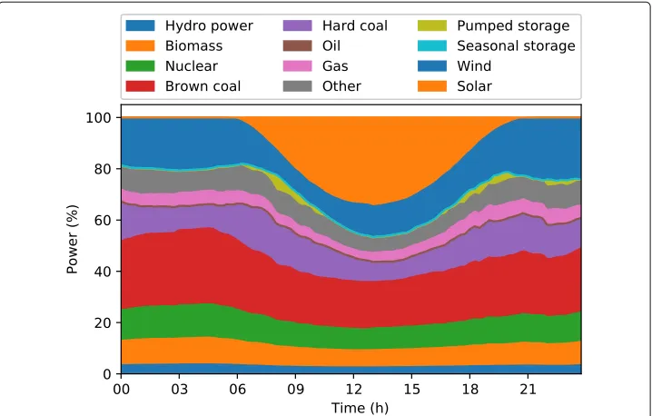
Given the generation mix of a power system and the hourly amount of energy generated per type of unit, it is possible to calculate the dynamic CO2-equivalent intensity factor associated to one kWh of energy that an end-user buys from the grid. Stoll et al. present a method to calculate the hourly values based upon the amount of hourly electricity gen-erated and traded, and the emission factors of the sources (Stoll et al.2014; Nilsson et al.2017). In this study, we use the data available for the German electricity grid on the European Network of Transmission System Operators for Electricity (ENTSO-E) Trans-parency Platform (Entsoe TransTrans-parency Platform). In Fig.1, one can see an example of hourly generation mix for one day in July 2017, when one kWh produced in a very windy and sunny hour (e.g., at 12.00 pm) was “cleaner” than a unit of energy produced during night hours (e.g., 01.00 am), when there was no solar production. Considering the emis-sion factors in Table1, the dynamic CO2-equivalent intensity factor of the German grid varied in 2017 between 113 gCO2eq/kWh and 533 gCO2eq/kWh.

Emission factors for several kinds of sources are given in (Weisser2007; Kono et al.

2017; Edenhofer et al. 2011); it is possible to quantify the emissions over all stages of electricity production, from production of infrastructure, technologies, and fuel, to con-version to electricity, to waste management. For the sake of completeness, we consider the

Table 1Life-cycle GHG emission for power plants, expressed in gCO2eq/kWh

Biomass Solar PV Wind onshore Wind offshore Geothermal Pumped-Storage

71 43 8 9 45 * 34

Run-of-the-river Reservoir Nuclear Lignite Coal Coal-derived gas

4 9 11 820 800 800

Gas Oil Waste Other

400 520 690 ** 247

The main source for these values is (Weisser2007). Values marked with * are taken from (Edenhofer et al.2011), and those marked with ** are from (Johnke2009). Since it is not specified which sources are included in “Other”, the life-cycle GHG emission factor for this category is calculated as the mean value of all other known factors

emission values related to a life-cycle assessment. In particular, Weisser (Weisser2007) reviews and compares the life-cycle GHG emissions for present andfuture/advanced

technologies, the latter referring to best performance power plants with increased effi-ciency in a realistic 2010-2020 scenario. In Table1, we report the emission factors used in this study. When available, we use the data for future/advanced technologies (i.e., for lignite, hard coal, gas, solar, and wind), otherwise mean values are considered. The areas in which improvements in GHG emissions may occur in future depend on the type of power plants. For instance, power plants burning fossil fuels are likely to be equipped with improved abatement technologies and burners; on the other hand, the development of new materials will reduce the emissions in the construction phase of wind turbines and solar panels (Weisser2007).

According to the criteria used by ENTSO-E in drawing itsMonthly Statistics Reports

(Statistics and Data), we use the generation data available for the third Wednesday of four months of 2017, namely January, April, July, and October. Moreover, we include the data for May, 8th 2016, a sunny and windy Sunday when more than 50% of energy was produced by renewable plants, covering more than 90% of power demand in a couple of hours (Craig Morris). For each day, we calculate the dynamic CO2-equivalent intensity factor for the German gridEFe,tas follows:

EFe,t=

ppEt,pp·EFpp

ppEt,pp

(1)

whereEt,ppis the energy produced by power plantppin time stept, andEFppis the

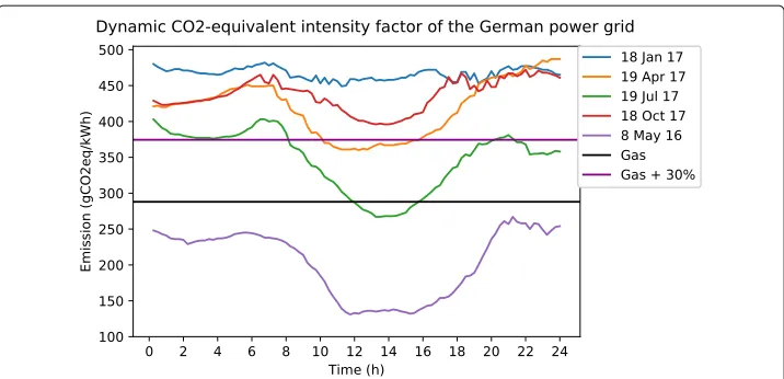
life-cycle GHG emission factor of power plant pp. The resulting dynamic CO2-equivalent intensity factors are displayed in Fig.2. These values are compared to the emission factor of burning gas for heating purposes, i.e., 288 gCO2eq/kWh (Edenhofer et al.2011), and to the equivalent value increased by +30%, corresponding to the increasing in appliances’ consumptions when using gas instead of electricity as main source (Mauser et al.2016; Mauser et al.2017). When appliances are using gas or hot water, in fact, additional losses have to be taken into account, such as heat dissipation. This study does not consider the German import of the electricity from the neighboring countries, since in the whole year 2017 it amounted to 15.6 TWh, less than 3% of the total generation.

Appliances: energy demand and user’s preferences

Residential appliances can be distinguished according to the energy carriers they require (Mauser et al.2015) and the operational characteristics (Chen et al.2012).

Fig. 2Dynamic CO2-equivalent intensity factors for five representative days, given German generation mix data

the other hand, some devices can be supplied by multiple energy carriers, namely hot water, electricity, and gas, which are used alternatively or in parallel to operate (Mauser et al.2017). This type of devices is referred to ashybridand the potential benefit of their application have recently gained interest in literature (Mauser et al.2015; Mauser et al.

2016; Stamminger et al.2008). Although the idea of suppling from different energy carri-ers may sound far from reality, there are solutions already commercially available. Some dishwashers and washing machine can be connected to a hot water supply, drastically reducing the power demand, as the water is no longer internally heated (Stamminger et al.2008). Gas clothes dryers heat the air by burning gas, while a hot water tumble dryer is equipped with a water-air heat exchanger (Stamminger et al.2008). Additionally, dual-fuel cookers are widely used, combining gas hobs and electric ovens; although not yet commercially available, it could be possible to combine electricity and gas in the same cooking device (Mauser et al.2017). Moreover, water can be boiled in an electric kettle or in a kettle (or a pot) placed on an electric hob, as well as in a kettle placed on a gas hob (Oberascher et al.2011). The hot water needed for space heating and bathing can be provided by electric heaters as well as gas-burning boilers. An innovative alternative is being developed by Nerdalize (Nerdalize), which uses cloud servers as preheating systems in homes, reducing at the same time the consumptions of gas for house heating and of electricity for server cooling.

Additionally, the devices are distinguished in shiftable and on-demand. For the former type, the user selects a time window during which the device is supposed to run and conclude its pre-selected task, which corresponds to a power demand profile. The latter type includes not-shiftable devices that have to be switched on and off when needed.

Demand profile and user’s preferences

The total energy consumptions per operation cycles of each appliance are summarized in Table2, while an example of the electricity-only and multi-carrier demand profiles of a hybrid appliance (i.e., dishwasher) are displayed in Figs.3and4, respectively. The con-sumption data are derived and adjusted from (Wood and Newborough2003; Stamminger et al.2008; Mauser et al.2017). When using gas or hot water heated by the gas-burning boiler, consumption are assumed to be +30% higher, due to additional distribution losses, heat dissipation, and water-air heat exchange process (Mauser et al.2015; Mauser et al.

2017). Therefore, the electrical efficiency of a hybrid appliance aisηe,a = 1, while the

thermal efficiency isηh,a =0.77. Operation preferences set by the user are summarized

in Table3.

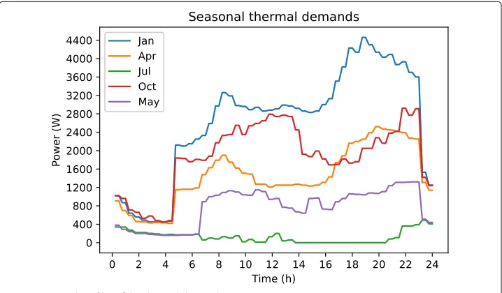
The daily thermal demand (Fig.5) is modeled with five seasonal curves, which are gen-erated by using the MERIT tool (University of Strathclyde). Electric heater systems for both space and water heating are assumed to have an electrical efficiencyηe,SW = 0.98

(Alahäivälä et al.2015; Heinen et al.2016); when a high-efficiency gas-fired boiler is used, we consider a total thermal efficiency of the heating systemηh,SW =0.89, as a results of

the boiler efficiencyηB=98% (Heinen et al.2016) and an increase in the thermal load by 10% due to losses in the distribution (Maivel and Kurnitski2014).

Problem formulation

The optimal scheduling problem is modeled as a mixed-integer linear programming (MILP) problem, where the variables to be determined are the status (on=1 or off=0) of each device in each time step with respect to the different energy carriers. In particular,

δa,s,t,l is a binary variable indicating the operation status (0 or 1) of appliancea

requir-ing level l from the energy carriers at time stept. We simulate a 24 h horizon with 15-min time steps. Five days with different thermal load are simulated with four possible configurations.

We assume that CO2signals with quarterly resolution are known at the beginning of the simulated day, so that the supply and demand can be optimally scheduled for the whole day. This may actually not be the case in a real scenario, where data about the German generation mix are available with a couple of hours of delay. However, it is possible to

Table 2Energy consumptions per operation cycle of household hybrid appliances

Appliance Electricity-only mode Hybrid mode (electricity + hot water/gas)

kWh kWh

HB 1.650 0.006 + 2.135 (gas)

OV 2.500 0.150 + 3.055 (gas)

KT 0.183 0.0015 + 0.234 (gas)

DW 1.193 0.160 + 1.343 (hot water)

WM 0.888 0.213 + 0.878 (hot water)

TD 2.460 0.400 + 2.808 (hot water)

Fig. 3Example of demand profiles of a hybrid appliance (DW): electricity only (Stamminger et al.2008)

forecast such data with accuracy of around 10%, for example by using those of the previ-ous 24 h as suggested in (Kristinsdóttir et al.2013). Moreover, according to the proposed problem formulation, devices may not be scheduled to the next day and thus may not benefit from low emissions after the evening peak. To contain the effects of such limita-tion, main shiftable loads (i.e., DW, WM, and TD) are assumed to have a 24 h operation window and thus they may be scheduled during night period.

Objective function

The dailyCO2emissions to be minimized are defined as follows:

min

t· 96

t=1

EFe,t

a∈A

Pa,e,t ηe,a +

EFh

a∈A

Pa,h,t ηh,a +

EFe,t

a∈A

Pa,eh,t ηe,a

(2)

Table 3Summary of user’s preferences

HB OV KT* DW WM TD SW

Operation on-demand

Startαa 19:00 12:00 7:00 20:00 09:00 14:00 00:00

Endβa 20:00 13:00 7:15 22:00 11:00 16:00 24:00

Durationγa 4 4 1 8 8 8 96

Shifting in time

Startαa 19:00 12:00 7:00 00:00 00:00 00:00 00:00

End_βa 20:15 13:15 7:30 24:00 24:00 24:00 24:00

Durationγa 4 4 1* 8 8 8 96

The durationγais expressed in time steps, where each time step is a quarter of an hour. The kettle is assumed to operate 5 min out of one time step

wherePa,e,tis the power consumption of applianceaat time steptwhen operating in

electricity-only mode, whilePa,h,t, andPa,eh,tare the heat and electricity demands when

operating in hybrid mode.t is the duration of one time step, i.e., a quarter of an hour .With respect to the kettle, we consider a 2200 W-device that operates for 5 min out of one time step. By doing so, the energy consumption is realistically set at 183 Wh (Wood and Newborough2003) and the emissions are calculated accordingly.

The power and/or heat demands at each time steptfor each applianceaare defined as follows:

Pa,s,t=

γa

l=1

δa,s,t,l·Pa,s,l ∀a∈A,∀s∈S,∀t∈T (3)

wherePa,s,lis the demand of sourcesequal to levellfor appliancea,Tis the set of time

steps, andSis the set of energy carriers (electricity-onlye, heath, electricity in hybrid modeeh). Given the demand profile of a device during its operation, the required power or heat in each quarter of hour corresponds to a level l. We defineAas the set of all appliances, which does not include the thermal load indicated asSW.

The objective function is subjected to several constraints as described next.

Constraints

Hybrid appliances can work in electricity-only or hybrid mode, that means, they require electricity and/or hot water/gas in a time stept(Equation4). Additionally, when work-ing in hybrid mode, both electricity and heat have to be (un)used at the same time (Equation5)

s∈S

γa

l=1

δa,s,t,l≤2 ∀a∈A,∀t∈T (4)

δa,h,t,l=δa,eh,t,l ∀a∈A,∀t∈T,∀l∈[ 1,γa] (5)

The thermal load can work in electricity-only or gas-only modes, hence in each time steptit can use one energy carrier at the most (Equation6) and no hybrid operation is possible (Equation7). Moreover, one single level of demand can be satisfied at each time step.

s∈S

γSW

l=1

δSW,s,t,l≤1 ∀t∈T (6)

δSW,eh,t,l=0 ∀t∈T,∀l∈[ 1,γSW] (7)

The consumer sets an operation window for each appliance [αa,βa], and no operation

is allowed outside this interval (Equation8). Additionally, all appliances have to com-plete their operation of lengthγa within the operation window and they are assumed

to run in non-interruptible mode. Moreover, the levels of demand have to be satisfied consecutively. These constraints are summarized in Equation9.

δa,s,t,l=0 ∀a∈A∪SW,∀s∈S,∀l∈[ 1,γa] ,∀t∈T\[αa,βa] (8)

δa,s,t,l=δa,s,t−1,l−1 ∀a∈A∪SW,∀s∈S,∀l∈[ 1,γa] ,∀t∈[αa,βa] (9)

The total power imported from the grid is limited toPe,MAX = 8 kW in electricity-only mode and to 3 kW in the hybrid one.

a∈A∪SW

s∈S\h

Pa,s,t≤Pe,MAX ∀t∈T (10)

Similarly, the output of the gas-burning boiler is limited toPb,MAX = 15 kW. We indi-cate withAhwthe set of appliances using hot water in hybrid mode, namely the washing

machine, the dryer, and the dishwasher.

a∈Ahw∪SW

Pa,h,t≤Pb,MAX ∀t∈T (11)

Moreover, we assume that the dryer has to run after the washing machine ends, hence:

t−1

τ=1

γWM

l=1

s∈S\eh

δWM,s,τ,l≥γWM·

s∈S\eh

δTD,s,t,0 ∀t∈T (12)

Simulation and evaluation

Configurations

Four possible configurations with increasing flexibility are compared:

• Case A: the whole energy demand is supplied by the electricity grid. We assume an efficiencyη=1for all electric appliances andηR=0.98for electric (water) heaters. Loads have to run on-demand, without the possibility of being shifted in time.

• Case B: all loads are running in hybrid-mode and the thermal load is supplied by a gas-burning boiler. We assume that appliance’s consumptions running in

hybrid-mode are 1.3 times higher. The gas-burning boiler hasηB=0.98and the thermal load is assumed to be 1.1 times higher than in electricity-only mode, due to losses in the distribution system. Loads have to run on-demand, without the possibility of being shifted in time.

• Case C: appliances are optimally scheduled with respect to the energy carriers, according to CO2signals. Loads have to run on-demand, without the possibility of

being shifted in time.

• Case D: appliances are optimally scheduled with respect to the energy carriers and their operation can be shifted in time, according to user’s preferences.

According to these configurations, some constraints may have to be added to the general model defined in the previous section.

Extra constraints

When all appliances run in electricity-only mode (Case A), it is not possible to use gas to produce hot water or heat, hence Equation13is added to the model:

δa,h,t,l =0 ∀a∈A∪SW,∀l∈[ 1,γa] ,∀t∈T (13)

On the other hand, when all appliances are running in hybrid-mode and the thermal load is supplied by the gas-burning boiler (Case B), Equation14is added:

δa,e,t,l=0 ∀a∈A∪SW,∀l∈[ 1,γa] ,∀t∈T (14)

Implementation

The MILP model is implemented in Python 2.7 and solved by GUROBI optimizer (Gurobi), which provides a free academic version. We use the Beautiful Soup package (Beautiful) for pulling data out of XML files provided by the ENTSO-E platform. In par-ticular, we use data referred to asActual Generation per Production Type, that is described in (Detailed Data Description) as the “aggregated generation output per market time unit and per production type”. For data analysis and data structure, we use the Numpy pack-age (Numpy V1.11.3.) and the Pandas packpack-age (Pandas V0.20.3.). Results are stored and manipulated by using the H5py package (H5py V2.7.0.), while MatPlotLib (MatPlotLib V2.0.2.) is used to visualize the results. For these simulations, the configuration of the computer hardware used is: CPU Intel®Core™i7-6600U, 2.60 GHz, with 16 Gb of RAM running Windows 10 64 bit. Simulating the scheduling of one day takes 4 to 5 s.

Results

Table 4Total daily carbon emissions [kg] and variations in percentage

Case 18/01/17 19/04/17 19/07/17 18/10/17 8/05/16

A 34.4 18.8 4.1 24.1 5.4

B 24.2 (-30%)* 14.8 (-21%)* 4.5 (+10%)* 18.3 (-24%)* 9.4 (+74%)* C 24.2 (-30%)* 14.8 (-21%)* 3.9 (-5%)* 18.3 (-24%)* 6.3 (+17%)*

D 24.2 (<1%)** 14.7 (<1%)** 3.7 (-5%)** 18.2 (<1%)** 5.8 (-8%)**

*: reference case is Case A; **: reference case is Case C

The hybrid operation (Case B) is the closest one to the optimal solution in 3 days out of 5, namely 18 January, 19 April, and 18 October, when the dynamic CO2-equivalent intensity factor of the electricity is indeed significantly higher than the one associated with burning gas in the boiler. In these cases, although using hot water and gas implies a +30% increase in the loads’ consumptions, switching from electricity to another energy carrier enables to reduce equivalent carbon emissions on average by 25%. Looking at Case C on 19 April, the loads running between 10 am and 16 am, namely the oven and the dryer, are scheduled to run in electricity-only mode, as running in hybrid mode with 1.3 times higher consumptions would increase the equivalent carbon emissions. As one can see in Fig.2, the equivalent emission factor of the boiler due to the increasing in consumption is, indeed, slightly higher than the hourly CO2-equivalent intensity factor of electricity. When running in hybrid mode, shifting loads in time has a minor impact on the total emissions (Case D), due to gas-burning boiler emissions being constant during the day.

On the summer day and on the 8thof May 2016, the results show that the hybrid opera-tion would not be the most sustainable one. In these two days, indeed, the electricity-only mode scores the best; on 19 July, the carbon emissions are reduced by 9%, when com-pared to the hybrid mode. Additionally, there is a further improvement of 5% by choosing the energy carriers for the different loads with the proposed algorithm (Case C), as the thermal load is supplied by the boiler instead of by importing electricity. Moreover, shift-ing loads’ operation in time enable a further reduction in carbon emission of -5% when compared to the optimal scheduling with on-demand operation. In particular, all shiftable appliances run between 11.30 am and 4 pm, when renewable sources have major impact on the generation mix. Overall, between the worst (Case B) and the best scenario (Case D), the proposed scheduling method enables around 18% of carbon savings.

The 8thof May 2016 is, as expected, a particularly benevolent scenario, as the dynamic CO2-equivalent intensity factor of the grid is very low when compared to the average value of 353 gCO2eq/kWh for the German grid, when calculated with the source emission factors summarized in Table1. The most sustainable solution is achieved in Case A, when all loads are supplied by the electricity grid, up to 11 kW. In this scenario, the hybrid-mode would increase the emissions by 74%; the optimal schedule of Case C leads to +17% of CO2eq, due to the lower limit of the maximum power that can be imported from the grid. This limitation implies that the thermal load has to be supplied by the boiler, otherwise it would not be possible to turn on the appliances when required by the user. The results are partially improved in Case D by shifting some appliances in time, enabling around 8% of carbon savings. Considering 3 kW as maximum power limit, between the worst (Case B) and the best scenario (Case D), potential emission savings are around 38%.

Table 5Total energy consumptions over five days [kWh]

Case Electricity Heat

A 215 0

B 5 241

C 39 199

D 43 195

energy carrier. Therefore, energy consumptions are the lowest in Case A, where the losses are minor, as expected.

Conclusions

Given the increasing electricity residential consumptions and the global attention towards GHG emissions, we propose a method to optimally schedule household loads according to CO2signals, with the aim of minimizing the daily equivalent carbon emissions of a single house. Hybrid appliances and the daily thermal load can use electricity imported from the grid, natural gas, or hot water produced in a gas-burning boiler, and, eventually, they can be shifted in time. The problem is formulated as a mixed integer linear problem, where the variables to be determined are binary and indicate the operation status of the appliances requiring a certain level of power or heat from the different energy carriers in each time step. The results show that the proposed algorithm allows to schedule the household loads by significantly reducing the carbon emissions. When the contribution of renewable sources in the generation mix is low, using multiple energy carriers, namely gas, hot water, and electricity, to supply the household appliances and the thermal load can reduce carbon emissions up to 30%, on a winter day. On the other hand, windy and sunny days can benefit more from a scheduling mainly based on electricity, although the maximum power importable from the grid can limit the carbon savings. This is a realis-tic condition for many European countries, such as Italy, where exceeding this limit leads to an automatic load shedding, and France, where users pay a subscription according to their expected maximum power demand. In general, shifting loads in time has a smaller effect; when the hybrid-mode is to be preferred, emission savings are marginally affected by the variability in the dynamic CO2-equivalent intensity factor of the electrical grid, as the main energy carriers are hot water and gas, whose emission factor is constant. When the loads are mainly using electricity, shifting their operations in time while fulfilling the user’s preference can reduce the emissions up to around 8%. Overall, switching from a single-carrier mode to a multi-carriers one and vice versa can successfully enable up to 74% equivalent CO2emissions reduction. The good performance of the software in terms of run-time means that it can be used for modeling a larger group of households, and it is suitable for real-time scheduling. Future works include a more detailed user’s model; in particular, we will include some kind of thermal storage and we will consider the load pro-files available on LoadProfileGenerator (Noah Pflugradt), which can simulate the energy demand of several types of German household.

Abbreviations

Funding

This work is supported by the Netherlands Organization for Scientific Research under the NWO MERGE project, contract no. 647.002.006 (www.nwo.nl). Publication costs for this article were sponsored by the Smart Energy Showcases - Digital Agenda for the Energy Transition (SINTEG) programme.

Availability of data and materials

All data generated and analysed during the current study are available from the corresponding author on reasonable request.

About this Supplement

This article has been published as part ofEnergy InformaticsVolume 1 Supplement 1, 2018: Proceedings of the 7th DACH+ Conference on Energy Informatics. The full contents of the supplement are available online athttps:// energyinformatics.springeropen.com/articles/supplements/volume-1-supplement-1.

Authors’ contributions

Laura Fiorini designed the study, performed the data analysis, and wrote the manuscript. Marco Aiello discussed the results, reviewed and finalized the manuscript. All authors have read and approved the final manuscript.

Competing interests

The authors declare that they have no competing interests.

Publisher’s Note

Springer Nature remains neutral with regard to jurisdictional claims in published maps and institutional affiliations.

Author details

1_{Department of Distributed Systems, University of Groningen, Nijenborgh 9, 9747 AG Groningen, The Netherlands.} 2_{Department of Smart Energy Systems and Services, University of Stuttgart, Universitätsstraße 38, 70569 Stuttgart,}

Germany.

Published: 10 October 2018

References

Alahäivälä A, Heß T, Cao S, Lehtonen M (2015) Analyzing the optimal coordination of a residential micro-CHP system with a power sink. Appl Energy 149:326–337

Beautiful Soup V4.6.0.https://www.crummy.com/software/BeautifulSoup/bs4/doc/#. Accessed 07 Mar 2018

Braun M, Dengiz T, Mauser I, Schmeck H (2016) Comparison of multi-objective evolutionary optimization in smart building scenarios. In: European Conference on the Applications of Evolutionary Computation. Springer, Cham. pp 443–458 Chen Z, Wu L, Fu Y (2012) Real-time price-based demand response management for residential appliances via stochastic

optimization and robust optimization. IEEE Trans Smart Grid 3(4):1822–1831

Craig Morris Germany Nearly Reached 100 Percen Renewable Power on Sunday.https://energytransition.org/2016/05/ germany-nearly-reached-100-percent-renewable-power-on-sunday. Accessed 11 May 2016

Dahl Knudsen M, Petersen S (2016) Demand response potential of model predictive control of space heating based on price and carbon dioxide intensity signals. Energy Build 125:196–204

Detailed Data Description.https://docstore.entsoe.eu/Documents/MC%20documents/Transparency%20Platform/MOP/ DetailedDescriptionDocument.pdf. Accessed 30 July 2018

Edenhofer O, Pichs-Madruga R, Sokona Y, Seyboth K, Matschoss P, Kadner S, Zwickel T, Eickemeier P, Hansen G, Schlömer S, von Stechow C (2011) IPCC, 2011: Summary for Policymakers. In: IPCC Special Report on Renewable Energy Sources and Climate Change Mitigation. Cambridge University Press, Cambridge. p 246

Entsoe Transparency Platform.https://transparency.entsoe.eu/. Accessed 07 Mar 2018

European Commission Buildings.https://ec.europa.eu/energy/en/topics/energy-efficiency/buildings. Accessed 07 Mar 2018

Gurobi Optimizer V7.0.2.http://www.gurobi.com/. Accessed 07 Mar 2018 H5py V2.7.0.https://www.h5py.org/. Accessed 07 Mar 2018

Haines V, Lomas K, Murray T, Ian R, Tracy N, Monica G (2010) How Trends in Appliances Affect Domestic CO2 Emissions : A Review of Home and Garden Appliances. Dep Energy Cli Chang March 2010:1–6. Department of Energy and Climate Change (DECC)

Heinen S, Burke D, O’Malley M (2016) Electricity, gas, heat integration via residential hybrid heating technologies - An investment model assessment. Energy 109:906–919

Johnke B (2009) Emissions From Waste Incineration. In: Good Practice Guidance and Uncertainty Management in National Greenhouse Gas Inventories. pp 455–468.https://www.ipcc-nggip.iges.or.jp/public/gp/bgp/5_3_Waste_ Incineration.pdf

Kono J, Ostermeyer Y, Wallbaum H (2017) The trends of hourly carbon emission factors in Germany and investigation on relevant consumption patterns for its application. Int J Life Cycle Assess 22(10):1493–1501

Kristinsdóttir AR, Stoll P, Nilsson A, Brandt N (2013) Description of climate impact calculation methods of the CO2e-signal for the Active House project. Tech Rep.http://kth.diva-portal.org/smash/record.jsf?pid=diva2:651166. Accessed 08 May 2018

Maivel M, Kurnitski J (2014) Low temperature radiator heating distribution and emission efficiency in residential buildings. Energy Build 69:224–236

MatPlotLib V2.0.2.https://matplotlib.org/. Accessed 07 Mar 2018

Mauser I, Müller J, Allerding F, Schmeck H (2016) Adaptive building energy management with multiple commodities and flexible evolutionary optimization. Renew Energy 87:911–921

Mauser I, Müller J, Schmeck H (2017) Utilizing Flexibility of Hybrid Appliances in Local Multi-modal Energy Management. In: Proceedings of the 9th international conference on energy efficiency in domestic appliances and lighting (EEDAL ’17)-Part III. Publications Office of the European Union, Luxemburg. pp 1282–1297

Nerdalize.https://www.nerdalize.com. Accessed 30 July 18

Nilsson A, Stoll P, Brandt N (2017) Assessing the impact of real-time price visualization on residential electricity consumption, costs, and carbon emissions. Resour Conserv Recycl 124:152–161

Noah Pflugradt Load Profile Generator.http://www.loadprofilegenerator.de. Accessed 08 May 2018 Numpy V1.11.3.http://www.numpy.org/. Accessed 07 Mar 2018

Oberascher C, Stamminger R, Pakula C (2011) Energy efficiency in daily food preparation. Int J Consum Stud 35(2):201–211 OECD IEA (2015) Energy and Climate Change: World Energy Outlook Special Report. International Energy Agency, Paris Pandas V0.20.3.https://pandas.pydata.org/. Accessed 07 Mar 2018

Paridari K, Parisio A, Sandberg H, Johansson KH (2015) Robust Scheduling of Smart Appliances in Active Apartments With User Behavior Uncertainty. IEEE Trans Autom Sci Eng 13(1):247–259

Siano P (2014) Demand response and smart grids - A survey. Renew Sust Energ Rev 30:461–478

Sou KC, Kördel M, Wu J, Sandberg H, Johansson KH (2013) Energy and CO2efficient scheduling of smart home appliances. In: 2013 European Control Conference (ECC). IEEE, Zurich. pp 4051–4058

Statistics and Data.https://electricity.network-codes.eu/publications/statistics-and-data/. Accessed 08 Mar 2018 Stamminger R, Broil G, Pakula C, Jungbecker H, Braun M, Rüdenauer I, Wendker C (2008) Synergy potential of smart

appliances. Citeseer.http://citeseerx.ist.psu.edu/viewdoc/download?doi=10.1.1.378.4289&rep=rep1&type=pdf

Stocker TF, Qin D, Plattner G-K, Tignor M, Allen SK, Boschung J, Nauels A, Xia Y, Bex V, Midgley PM (2014) IPCC, 2013: Climate Change 2013: The Physical Science Basis. Contribution of Working Group I to the Fifth Assessment Report of the Intergovernmental Panel on Climate Change. Cambridge University Press, Cambridge

Stoll P, Brandt N, Nordström L (2014) Including dynamic CO2 intensity with demand response. Energy Policy 65:490–500 University of Strathclyde Demand Profile Generators.https://www.strath.ac.uk/research/energysystemsresearchunit/.

Accessed 08 May 2018

Weisser D (2007) A guide to life-cycle greenhouse gas (GHG) emissions from electric supply technologies. Energy 32(9):1543–1559

Wood G, Newborough M (2003) Dynamic energy-consumption indicators for domestic appliances: Environment, behaviour and design. Energy Build 35(8):821–841

Submit your manuscript to a

journal and benefi t from:

7Convenient online submission

7Rigorous peer review

7Immediate publication on acceptance

7Open access: articles freely available online

7High visibility within the fi eld

7Retaining the copyright to your article