Persistent inter‐industry wage differences: rent sharing and opportunity costs

O R I G I N A L R E S E A R C H

Open Access

Persistent inter-industry wage differences: rent

sharing and opportunity costs

John M Abowd

, Francis Kramarz

, Paul Lengermann

, Kevin L McKinney

and Sébastien Roux

*Correspondence: john.abowd@cornell.edu 1_{School of Industrial and Labor} Relations, Cornell University, US Census Bureau, CREST, IZA, and NBER, 261 Ives Hall, Ithaca, NY 14853, USA

Full list of author information is available at the end of the article

Abstract

We reconsider the potential for explaining inter-industry wage differences by decomposing those differences into parts due to individual and employer

heterogeneity, respectively. Using longitudinally linked employer-employee data, we estimate the model for the United States and France. The part arising from individual heterogeneity can be theoretically and empirically related to the worker’s opportunity wage rate. The part arising from employer heterogeneity can similarly be related to product market quasi-rents and relative bargaining power. We find that these two variables are highly correlated with both parts of the differential in France. Although the U.S. inter-industry wage differentials are strongly correlated with those in France, the decomposition is more nuanced in the American data, where the opportunity wage rate and the product market conditions are related to both the personal and employer heterogeneity.

JEL codes: J31, J50, L10

Keywords: Inter-industry wage differentials, Matched employer-employee data, Quasi-rents

1 Introduction

One of the most pervasive and difficult to explain phenomena in economics is the persistence of inter-industry wage differences for measurably similar workers. Some explanations predict that most of the variation is due to the persons employed in the industry, whose opportunity wage rates are similarly high or low. Other explanations predict that most of the variation is due to differential firm or industry compensation policies that do not follow the individual from job to job. Economists’ ability to distin-guish among these explanations has been hampered by the lack of appropriate matched, longitudinal employer-employee data. The arrival of such data has produced a resur-gence of interest in some classic problems of labor economics for which both sides of the market–workers and firms–matter (see the survey on matched data sources and some early results in Abowd and Kramarz (1999a) or the international results contained in Haltiwanger et al. (1999)). Modeling techniques derived from those used in statistical genetics have been developed to address the econometric challenges (see Abowd and Kramarz (1999b), Abowd et al. (2002a), and the survey in Abowd et al. (2008)). On the theoretical side, Mortensen (2003) and Postel-Vinay and Robin (2002) developed their search-based models to address the possibilities that linked data provide. Shimer (2005)

developed an assignment model and Cahuc et al. (2006) developed a search friction model with bargaining that were partly inspired by some of the results contained in this literature in particular Abowd et al. (1999b) (AKM, hereafter).

In this paper, we take stock of these developments to reexamine the classic question of inter-industry wage differentials using longitudinal linked employer-employee data for the United States and France. Although this topic received a flurry of attention in the 1980s, Krueger and Summers (1987) and Krueger and Summers (1988) established the consistency of these differentials over time and across countries, the fundamen-tal question remained unresolved: are these differentials due to individual or employer components? Individual factors stay with the worker from job to job, whereas employer differences affect any worker who has a job with the firm. Because these two parts are directly interpretable in terms of economic models, it is important to apportion the inter-industry differentials into these person and employer parts. This can only be done using longitudinal linked employer-employee data (see AKM).

Krueger and Summers stressed factors related to the employer, such as compensation policy, as the primary explanation of the inter-industry differentials although their analy-sis showed that such factors were, at best, an incomplete explanation. Murphy and Topel (1987), on the other hand, stressed individual unmeasured differences as the primary cause of the wage differentials, although, once again, their data were incomplete. Dick-ens and Katz (1987) tried to explain the inter-industry wage differentials using a variety of measured individual and firm characteristics aggregated to the industry level; hence, their analysis was very much in the spirit we propose but they could not control for the unmeasured differences that we stress below. Gibbons and Katz (1992) attempted to explain the differential based on unobserved individual heterogeneity. Brown and Medoff (1989) focused their attention on the firm-size wage differential. They attempted to dis-tinguish between explanations based on individual heterogeneity and those based on firm level compensation policy. In related work Groshen (1991) examined the role of firm and establishment compensation policy heterogeneity on wage outcomes, generally.

What distinguishes this paper from the earlier work is our ability to simultaneously con-trol for unobservable individual and employer heterogeneity, which none of the papers cited in the previous paragraph could do, under statistical assumptions that are exactly comparable to the ones that underlie those papers. In particular, neither Krueger and Summers nor Murphy and Topel could not apportion the respective contributions of unmeasured individual and employer differences. None of their data sources had suffi-ciently large micro-data samples to permit analysis at the level of detail and precision that we report here.

proportions to individual and employer heterogeneity while firm-size wage differentials are due primarily to firm heterogeneity.

Both AKM and AFK used statistical approximations to estimate the decomposition of wage differentials into individual and employer components. Furthermore, these papers did not try to understand the origin of these differentials. In this article we apply exact methods from Abowd et al. (2002a) to the estimation problem and comparable data sources for both countries, some of them part of the recent effort of the U.S. Census Bureau Longitudinal Employer-Household Dynamics Program’s infrastructure file system (Abowd et al. (2009)). A model of bargaining power also allows us to present economic interpretations of our results.

The paper is organized as follows. In section 2 we present a simple economic model that we use to interpret our estimates. Then, in section 3, we briefly discuss our estima-tion methods as well as the framework necessary to understand the estimated person and firm components of the inter-industry wage differentials and relate them to the literature. Section 4 presents the American and French data sources and labor market institutions. Section 5 discusses the inter-industry wage differential results. In particular, and in con-trast to the previous literature, we try to directly measure economic variables correlated with these differentials. Section 6 concludes1.

2 A simple economic model

To give an economic interpretation to our estimates of person and firm effects in the context of inter-industry wage differentials, we use a simple equilibrium model of wage determination with imperfect competition. We posit a simple bargaining model of wages of which perfect competition is a special case. Let the wage be determined by

wi=xi+γ QRj(i)

Lj(i)

wherexdenotes the opportunity cost of time of workeri,QRandLare, respectively, the quasi-rent and employment of her employing firmj(i), andγ is the workers’ bargaining power. This formula is directly derived from a bargaining game where workers and firms bargain over employment and wages (the so-called strongly efficient bargaining; see, for example, Abowd and Lemieux (1993) and Cahuc et al. (2006)). Then, write

E[wi]=μw=μx+γ μQR L

assuming a constantγ. Next, rewrite worker’s opportunity wage as

xi=μx+ξi

and the firm’s quasi-rent as QR_j(i)

Lj(i) = μQR

L + ρj(i)

then

wi=μw+xi−μx+γ

QRj(i) Lj(i) −

μQR L

=μw

1+xi−μx

μ_w +γ

QRj(i) μ_wLj(i)−

μQR L μ_w

=μw

1+θi+γ ρj(i)

μw

where ρ_μj(i) w ≡

QRj(i) μwLj(i) −

μQR L

μw . So, we may write the first-order approximation of our wage bargaining equation in the following log-separable format:

lnwi≈lnμw+θi+ψj(i) (1)

whereθ_i≡ ξi

μw andψj(i)≡ γj(i) ρj(i)

μw, which shows how to decompose the individual wage rate in to the opportunity cost of time lnμ_w+θ_i, the portable part of the wage rate, and the industry-specific share of the quasi-rent per worker,ψ_j(i).

Equation (1) has a simple format that can be directly estimated using the matched employer-employee data sources that we use. The additive decomposition helps us iden-tify our measures of person effects as opportunity wages and our measures of firm effects as real measures of the share of the quasi-rents that goes to workers. In the component, ψ_j(i), two elements matter. First,γj(i), workers’ bargaining power in industryj, is related to

union behavior and bargaining power in the firms of industryj. Second,ρ_μj(i) w =

QRj(i)

Lj(i) −μQR_L –the deviation of quasi-rent per worker in industryjfrom the quasi-rent per worker in the economy, is related to product market competition in the various industries.

In order to specify a formula for the quasi-rent per worker that can be applied to our aggregated data, we now show how to use equation (1) to correct industry total com-pensation for the component that is not portable, which is related toψj(i). Our analysis combines the insight of Abowd and Lemieux (1993) that only the opportunity cost of labor and capital inputs should be subtracted from industry revenue in computing a quasi-rent with that of Abowd and Allain (1996), who show that when the opportunity cost of time contains an individual-specific component, the average value of that component in the industry must be included in the opportunity cost of time measure. Since the estimation begins with equation (1), we exponentiate the approximation to obtain

wi=μwexp(θi+εi)exp

ψj(i)

where ε_i is the error of approximation, which is part of the statistical error in the estimation model. The expectation ofwiin industrykcan be written as

Ewi|j(i)∈Industryk

=μwexp(ψk)E

exp (θi+εi)|j(i)∈Industryk

.

When the residual variance of the log wage equation is small relative to the overall variance in wages, variance in wages, Kramarz (2008) shows that

Eexp(θi+εi)|j(i)∈Industryk

≈1+ ¯θ_k

whereθ¯_kis the industry-specific mean person effect2. Aggregating individual compensa-tion to the industry level gives the following formula for the average opportunity cost of time in the industry

μw

1+ ¯θk

≈ E

wi|j(i)∈Industryk

exp(ψ_k) . (2)

Using equation (2), we can express the quasi-rent per worker in industrykas a function of revenue per worker and the opportunity costs of capital and labor

QRk

Lk =

j∈IndustrykR

Lj,Kj

Lk −

rk Kk Lk −

xk (3)

= Rk Lk −

rk Kk Lk −

where QRk, Rk,Kk and Lk are industry total quasi-rents, revenue, capital and labor, respectively;rk is the opportunity cost of capital and expw(ψkk) is the opportunity cost of labor.

3 Statistical models and estimation

Our underlying statistical model can be expressed using the decomposition in AKM. Once this decomposition is estimated, we apply the formulae given therein to estimate the part of the inter-industry wage differential due to person and firm effects. A summary of the methodology is given in this section.

3.1 The AKM decomposition

The linear statistical model, taken directly from AKM, is specified as:

lnwit=xitβ+θi+ψJ(i,t)+εit (4)

wherexit denotes the time-varying variables,θithe pure person effect,ψJ(i,t) the pure firm effect, andε_itthe statistical residual. Note that the function J(i,t)gives the identifier for the dominant employer,j, of individualiat datet3. In full matrix notation we have

y=Xβ+Dθ+Fψ+ε (5)

whereXis theN∗×Pmatrix of observable, time-varying characteristics (in deviations from the grand means);Dis theN∗ ×N design matrix of indicators variables for the individual;Fis theN∗×Jdesign matrix of firm indicators variables for the firm effects for the employer at whichiworks at datet(Jfirms total);yis theN∗×1 vector of dependent data (also in deviations from the grand mean);εis the conformable vector of residuals; andN∗=N_i=1Ti. We assume thatεhas the following properties:

E [ε|X,D,F]=0

and

Cov [εi,εm|Di,Dm,Fi,Fm,Xi,Xm]= Ti

i,i=m 0, otherwise.

3.2 Industry effects4

represented as an employment-duration weighted average of the firm effects within the industry classificationk:

κ_k ≡ N

i=1 T

t=1

1(K(J(i,t))=k)ψJ(i,t) Nk

where

Nk≡ J

j=1

1(K(j)=k)Nj

and the function K(j)denotes the industry classification of firmj. If we insert this pure industry effect, the appropriate aggregate of the firm effects, into equation (4), then the equation becomes

yit =xitβ+θi+κK(J(i,t))+(ψJ(i,t)−κK(J(i,t)))+εit

or, in matrix notation as in equation (5),

y=Xβ+Dθ+FAκ+(Fψ−FAκ)+ε (6)

where the matrixA,J×K, classifies each of theJfirms into one of theKindustries; that is,a_jk = 1 if, and only if, K(j) = k. Algebraic manipulation of equation (6) reveals that the vectorκ,K×1, may be interpreted as the following weighted average of the pure firm effects:

κ≡(AFFA)−1AFFψ. (7)

The effect(Fψ−FAκ)may be re-expressed asMFAFψ, where the column null space of an arbitrary matrix,Z, is denotedMZ ≡I−Z

ZZ−Z, and()−is a computable g-inverse. Thus, the aggregation ofJfirm effects intoKindustry effects, weighted so as to be rep-resentative of individuals, can be accomplished directly by the specification of equation (6). Only rank(FMFAF)firm effects can be separately identified using unrestricted fixed-effects methods; however, there is neither an omitted variable nor an aggregation bias in the estimates of (6), using either of the class of methods discussed below. Equation (6) sim-ply decomposesFψinto two orthogonal components: the industry effectsFAκ, and what is left of the firm effects after removing the industry effect,MFAFψ. While the decom-position is orthogonal, the presence ofXandDin equation (6) greatly complicates the estimation using the fixed-effects techniques discussed in Appendix A (Additional file 1). When the estimation of equation (6) excludes both person and firm effects, as most of the literature has done, the estimated industry effect,κ_k∗∗, equals the pure industry effect, κ, plus the employment-duration weighted average residual firm effect inside the industry, givenX, and the employment-duration weighted average person effect inside the industry, given the time-varying personal characteristicsX:

κ∗∗=κ+(AFMXFA)−1AFMX(MFAFψ+Dθ )

which can be restated as

κ∗∗=(AFMXFA)−1AFMXFψ+(AFMXFA)−1AFMXDθ. (8)

The exact decomposition is entirely parallel to our theoretical model: the inter-industry wage differential is decomposed into two parts, a person and a firm component, both of which are properly adjusted for the presence of covariates. There are no ancillary, and unnecessary, orthogonality assumptions.

Notice that if industry effects,FA, were orthogonal to time-varying personal charac-teristics,X, and to non-time varying personal heterogeneity,D, so thatAFMXFA = AFFA, AFMXF = AFF, and AFMXD = AFD, the biased inter-industry wage differentials, κ∗∗, would simply equal the pure inter-industry wage differen-tials,κ, plus the employment-duration-weighted, industry-average pure person effect,

AFFA−1AFDθ, or

κ_k∗∗=κ_k+ N

i=1 T

t=1

1[ K(J(i,t))=k]θi Nk

whereNk ≡

i,t1[ K(J(i,t))=k].

3.3 Estimation of the fixed-effects model by direct least squares

The estimation methods proposed by AKM have been improved so that the statistical model can now be solved exactly for the fixed-effects case. The full solution and the asso-ciated identification analysis are reported in Abowd et al. (2002a), which is summarized in Additional file 1: Appendix A to the present paper5.

The nature of the identification of the firm effects can be more intuitively understood in terms of average treatment effects and local average treatment effects. The AKM decom-position identifies the average treatment effect of changing between two employers based on the contrast between the employer effects for those two employers, holding constant observables and individual heteogeneity. AKM uses the actual employment as the weights for this contrast, rather than just the movers, as would be the case for a local average treat-ment effect estimated by instrutreat-mental variables6. Further analysis of the identification in terms of average treatment effects can be found in Card et al. (2012).

4 Data description

We constructed very similar data for both the United States and France. In particular, we used administrative earnings reports from longitudinally linked employer-employee data to estimate the inter-industry wage differentials and their decomposition into person and firm effects. Then, we assembled comparable American and French industry-level data to explain the decomposition. Appendix B (Additional file 1) describes all of the data sources used7.

For the United States, we use a universe of statutory employees from seven states that were early participants in the Census Bureau’s Longitudinal Employer-Household Dynamics Program (see Abowd et al. (2002b); ALM, hereafter). Data cover the period from 1990 to 2001. There is no sampling of individuals or employers; however, federal employees are not covered by the database. Aggregate data from the Current Population Survey, the National Income and Product Accounts (assets and industry tables), and the Economic Censuses were integrated via the Standard Industrial Classification 1987.

Structure Survey, Ministry of Labor database on Agreements and Union Representatives, and the Bénéfices Industriels et Commerciaux/Bénéfices Réels Normaux (enterprise-level business data) were integrated via the Nomenclature d’Activités et de Produits 100. These data were also used in Abowd et al. (2006).

5 Comparison of institutions 5.1 The labor markets

For most analysts, the difference in the labor market situations between France and the United States is well summarized by Figure 1. This figure shows the employment-population ratio for the two countries for our sample period. The two countries have similar employment rates in the mid-seventies (65% and 67% , respectively). But there-after, they diverged. At the end of our sample period (the end of the nineties), the difference was close to 20 percentage points.

Since 1951, French industry has been subject to a national minimum wage (called the SMIC since the revisions to the relevant law in 1971) that is indexed to the rate of change in consumer prices and to the average blue-collar wage rate. The United States has also had a federal minimum wage during this same period. The American federal minimum wage is superseded by state-mandated rates during some years for some states. Figure 2 depicts the changes in the two (real) minima over the sample period. Exactly when the French SMIC started its very sharp increase (beginning of the seventies), the American minimum decreased rapidly. In the rest of the sample period, the French SMIC continued its increase, partly mandated by one-shot increases and partly by formulaic increases, whereas the American minimum wage fell until 1990 when it leveled off. Notice, however, that minimum wage rates delivered to the worker do not track the firm’s minimum labor costs. The structure of payroll taxes that augment wages as a part of labor cost has not

Figure 2 Comparison of French and United States real minimum wage indices.

changed substantially in the United States (during the period of our analysis) but it has changed in France. After a constant increase in payroll tax rates from the early 1970s, they dropped sharply in 1994 and even more so in the ensuing years (see Kramarz and Philippon (2001)) as a part of an explicit program to lower total labor costs for workers at the minimum wage.

workers ended up with an agreement as a result of these negotiations. Finally, the percent-age of the work force covered by some establishment or firm-level agreement on wpercent-ages is approximately 40% in 1992. The law required that the firm-level agreements could only improve the conditions stated in the industrial agreement, so that, over time, the firm-level agreements have become more important for wage determination than the industry agreements.

Although more than 90% of French workers are covered by industrial agreements throughout our analysis period (1976-1996), firm-level negotiations outpaced renego-tiations of industry-wide agreements in most industries. The regular increases in the national minimum wage (in particular those driven by the indexation to the average blue-collar wage rate) resulted in the lowest categories on the collective pay scales in most industry contracts for most occupations being below the national minimum by the beginning of the 1990s. When this occurs, it is the national minimum wage, and not the collectively bargained wage, that binds.

In the United States, the bargaining environment is very different from that prevailing in France. For this description as well as for the recent changes that affected this country, we rely on the work of Farber and Western (2001). Unionization in most sectors of the United States economy is governed by the National Labor Relations Act (NLRA), passed in 1935. While NLRA guaranteed the rights of employees (as distinct from workers or cit-izens, in general) to organize and bargain, it also established the procedure for a union to become the exclusive bargaining agent of a group of workers. The procedure starts when at least 30% of the workers in a work unit sign authorization cards. The union petitions the National Labor Relations Board (NLRB) in order to set up a representation election. The campaign takes place between the time of the petition and the election. Employers and unions both participate in the campaign. Once a union is certified and an initial con-tract negotiated, the jobs included in the bargaining unit become union jobs. Successor employers are normally bound to negotiate with the duly certified union unless there has been a decertification election.

Figure Four of Farber and Western (2001) shows the huge decrease in certification elec-tions that took place during the eighties. Furthermore, even for those elecelec-tions that took place, the union win rate also decreased sharply until 1975 and then leveled off at just less than 50% (Figure Five, id.). Not surprisingly, these facts, along with the decline in manufacturing employment generally, contributed to a sharp decline in the overall union-ization rate among private employers. Although the trend went in the opposite direction for public-sector employers, the overall unionization rate which went from 25% in 1974 to less than 13% in 1998. Although the private and the public sector union membership rates were equal in 1974 at 25%, the latter increased rapidly to 36% in 1980 and then stabilized but the former continuously decreased to 9.7% in 1998.

with the curvature of the quartic in experience implying a more hump-shaped profile in the U.S.. Finally, the gender wage gap in the initial year is roughly equal in both countries, although it decreases over the sample period in the U.S. and is basically stable in France during the eighties.

5.2 The product market

Apart from labor market institutions, the intensity of competition prevailing on the prod-uct market should affect wages according to the theory developed above because wages are the sum of an opportunity wage and a rent component. These rents are the prod-uct of workers’ bargaining power, an outcome of labor market institutions as described just above, and of the firms’ quasi-rent, an outcome of product market competition. Reg-ulations that affect product markets are more dispersed than labor market regReg-ulations. For instance, the American airline or banking industries were heavily regulated in the seventies. But these regulations were discarded during the 1980s and 1990s. The effects on labor market outcomes of such deregulation have been shown to be quite large10. To paraphrase the conclusion of Peoples (1998), the effect of deregulation was heavily tied to reductions in the labor costs that followed. In all the industries where labor earnings fell sharply, trucking or airline, employment increased dramatically. In industries where labor earnings fell slightly, such as telecommunications, employment was steady. Finally, in industries where earnings did not change, such as the railroad industry, employment sharply declined. Hence, our sample period for the United States is one of intense product market competition.

This is far from the case in France. Even though France, pushed by European insti-tutions, started in the 1990s to deregulate some industries, the process is far from completion. During our sample period, near monopolies operated in many industries. Air France (airlines), Seita (cigarettes), Electricité de France (energy), and Gaz de France (energy) are all examples of firms in which the State has a majority equity stake and there are no local competitors (even though France imports cigarettes and allows foreign air-lines to land in France). Entry into these industries was, and still is, heavily regulated. Surprisingly, it is also the case in many other apparently competitive industries, such as the retail trade, that entry regulations loomed and are still very important (see Bertrand and Kramarz (2002) for the detrimental effect of the Loi Royer on employment in the retail trade). Djankov et al. (2002) have also shown that entry regulations, as measured by requirements to starting a new business in France, are common, time-consuming and costly. This startup process takes 66 days and 16 different legal and administrative steps in France and only 7 days and 4 steps in the United States.

6 Basic results

Table 1 US, winners and losers

SIC Industry Raw Industry Industry Industry Average Average Wage Person Firm Differential Effect Effect

62 Security brokers, dealers, exchanges 0.659 0.393 0.258

46 Pipelines, except natural gas 0.625 0.094 0.475

29 Petroleum and coal products 0.478 0.109 0.345

81 Legal services 0.471 0.236 0.230

48 Communications 0.460 0.123 0.346

49 Electric, gas, and sanitary services 0.445 0.095 0.358

13 Oil and gas extraction 0.437 0.108 0.285

38 Instruments and related products 0.411 0.137 0.280

89 Miscellaneous services 0.409 0.136 0.227

28 Chemicals and allied products 0.407 0.126 0.303

83 Social services −0.296 −0.199 −0.102

53 General merchandise stores ₋0.303 ₋0.050 ₋0.241

79 Amusement and recreation services −0.312 −0.079 −0.249

72 Personal services −0.371 −0.160 −0.213

70 Hotels, rooming houses, camps, and lodging −0.385 −0.209 −0.186

23 Apparel and other textile products −0.402 −0.240 −0.142

58 Eating and drinking places ₋0.554 ₋0.161 ₋0.397

07 Agricultural services −0.568 −0.280 −0.316

01 Agriculture−crops −0.570 −0.293 −0.315

88 Private households −0.643 −0.219 −0.252

estimate of(AFMXFA)−1AFMXDθ, the average of the person effects within the indus-try adjusted forX. The column labeled “Industry Average Firm Effect” is an estimate of (AFMXFA)−1AFMXFψ, the average of the firm effects within the industry adjusted for X. The columns of these two tables serve as the dependent variables for the long-term statistical analysis performed in section 712.

An instructive way to summarize the results is to consider the industries with the largest positive and negative raw wage differentials. For the U.S. these “winners and losers” are summarized in Table 1. Notice that the industry with the largest raw differential is SIC 62 (security brokers, dealers and exchanges). This raw differential of 0.659 log points consists of two-thirds person effect and one-third firm effect. One can conclude that for whatever economic reasons, persons with high opportunity costs of time (largeθ_i) accumulate in this sector and, again for whatever economic reasons, firms in this sector pay more. SIC 62 has both high-wage workers and high-wage firms. Now consider the second largest “winner,” SIC 46 (pipelines, except natural gas). In this sector the large differential is is basically due to the presence of high-wage firms (largeψj). Consider now the “losers.” The biggest negative raw differential is in SIC 88 (private households), where more of the difference is due to firm effects than to person effects but the two both contribute substantially to the differential. SIC 83 (social services), on the other hand, is due two-thirds to the average person effect and one-third to the average firm effect.

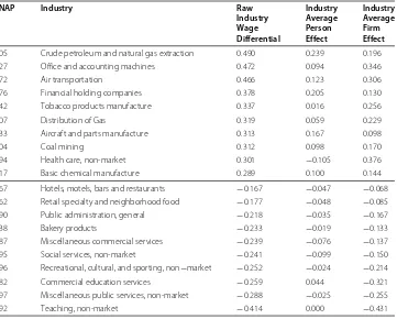
Table 2 France, winners and losers

NAP Industry Raw Industry Industry Industry Average Average Wage Person Firm Differential Effect Effect

05 Crude petroleum and natural gas extraction 0.490 0.239 0.196

27 Office and accounting machines 0.472 0.094 0.346

72 Air transportation 0.466 0.123 0.306

76 Financial holding companies 0.378 0.205 0.130

42 Tobacco products manufacture 0.337 0.016 0.256

07 Distribution of Gas 0.319 0.059 0.229

33 Aircraft and parts manufacture 0.313 0.167 0.098

04 Coal mining 0.312 0.098 0.170

94 Health care, non-market 0.301 −0.105 0.376

17 Basic chemical manufacture 0.289 0.100 0.144

67 Hotels, motels, bars and restaurants −0.167 −0.047 −0.068

62 Retail specialty and neighborhood food ₋0.177 ₋0.048 ₋0.085

90 Public administration, general −0.218 −0.035 −0.167

38 Bakery products −0.233 −0.019 −0.133

87 Miscellaneous commercial services −0.239 −0.076 −0.137

95 Social services, non-market −0.241 −0.099 −0.150

96 Recreational, cultural, and sporting, non₋market ₋0.252 ₋0.024 ₋0.214

82 Commercial education services −0.259 0.044 −0.321

97 Miscellaneous public services, non-market −0.288 −0.025 −0.255

92 Teaching, non-market −0.414 0.000 −0.431

government-ownership of the largest businesses (on the top of the wage distribution). Nevertheless, there are some big “winners.” The biggest is NAP 05 (crude petroleum and natural gas extraction) where the raw effect consists of about equal parts person and firm effects. The story is very different for the second “winner.” In NAP 27 (office and account-ing machines) most of the effect comes from the average firm effect. Similarly, NAP 72 (air transport) and NAP 42 (tobacco products) and NAP 07 (distribution of gas) all derive the bulk of their raw differential from the industry average firm effect. Interestingly, all of these industries contained large government-owned firms during the sample period. Among the “losers” the most striking feature is the compression of the industry aver-age person effects (especially in comparison with the U.S.), which is almost surely due to the SMIC. The largest “loser” NAP 92 (teaching, non-market) is a very small sector. The largest of the “loser” market sectors are NAP 67 (hotels, motels, bars and restaurants) and NAP 62 (retail specialty and neighborhood food), which employ 7% of the total workforce, have large negative raw differentials consisting of two-thirds firm effect and one-third person effect.

IZA

Journal

o

fL

abor

Economics

2012,

1

:7

Page

14

of

25

Table 3 Correlation of industry effects

France US

Raw Industry Industry Industry Raw Industry Industry Industry

Wage Average Average Firm Wage Average Average Firm

Differential Person Effect Effect Differential Person Effect Effect

France French Industry Weights

Raw Industry Wage Differential 1.0000 0.6110 0.9046 0.5783 0.4444 0.5689

Industry Average Person Effect 0.6110 1.0000 0.2549 0.4810 0.6337 0.2880

Industry Average Firm Effect 0.9046 0.2549 1.0000 0.3792 0.1655 0.4564

US US Industry Weights

Raw Industry Wage Differential 0.4914 0.3652 0.3630 1.0000 0.8167 0.9214

Industry Average Person Effect 0.2662 0.4631 0.0630 0.8167 1.0000 0.5382

the forces that sort person effects are not strongly correlated with the forces that sort firm effects.

7 Long term factors

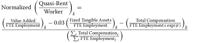
In order to implement the wage determination model embodied in equation (1), we esti-mated normalized quasi-rents per worker using the industry aggregate data described in Additional file 1: Appendix B14. The exact definition of the normalized quasi-rent per worker is for industrykis:

Normalized

Quasi-Rent Worker

k

= (9)

Value Added FTE Employment

k−0.03

Fixed Tangible Assets FTE Employment

k−

Total Compensation FTE Employment×exp(ψ)

k

Total Compensation

FTE Employment

where the appropriate, country-specific, value has been used for each of the variables noted in the general formula. Notice that the division of the total compensation per FTE employee by exp(ψ_k)removes the non-portable part of the compensation from the opportunity cost of labor as shown in the derivation of equation (3)15. As is clear from the formula, we assumed a 3% real opportunity cost of capital. Our definition differs in two important respects from the one used by Abowd and Lemieux. First, we normalize the quasi-rent per work by dividing by the economy-wide average compensation, which is a constant across sectors, in order scale the effects in France and the United States to be unit free. Second, we correct the opportunity cost of time, computed as_{FTE Employment}Total Compensation_×exp(ψ), for the variation in average person effects across industries, a measure that Abowd and Lemieux could not estimate. Although the formula uses exp(ψ ), equation (2) shows that the result is exactly the average opportunity cost of time for workers in the industry. This adjustment is similar to the one used by (Abowd and Allain 1996) although they worked with firm-level data.

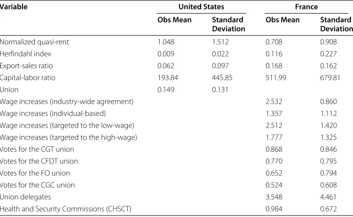
Table 4 presents a summary of the variables we use to account for the raw inter-industry wage differentials and their component industry-average person and firm effects in our statistical analysis of the long run factors correlated with these effects. The exact con-struction of all these variables is precisely described in the data Appendix (Additional file 1).

Table 5 shows the results with no controls other than the variables listed16. The first six columns present estimates for the United States. The last six columns present equivalent results for France. For each country, we estimate three specifications of the explanatory variables. For industryk, the industry-average person and firm effects,θ_k andψ_k consti-tute our two endogenous variables in each specification. These average person and firm effects are estimated using the methods described in section 3. In each case, we include a measure of the (normalized) industry quasi-rent per worker.

Table 4 Descriptive statistics of independent variables

Variable United States France

Obs Mean Standard Obs Mean Standard Deviation Deviation

Normalized quasi-rent 1.048 1.512 0.708 0.908

Herfindahl index 0.009 0.022 0.116 0.227

Export-sales ratio 0.062 0.097 0.168 0.162

Capital-labor ratio 193.84 445.85 511.99 679.81

Union 0.149 0.131

Wage increases (industry-wide agreement) 2.532 0.860

Wage increases (individual-based) 1.357 1.112

Wage increases (targeted to the low-wage) 2.512 1.420

Wage increases (targeted to the high-wage) 1.777 1.325

Votes for the CGT union 0.868 0.846

Votes for the CFDT union 0.770 0.795

Votes for the FO union 0.652 0.794

Votes for the CGC union 0.524 0.608

Union delegates 3.548 4.461

Health and Security Commissions (CHSCT) 0.984 0.672

Indeed, union strength is highly correlated to the firm effect and not the person effect in both countries.

The two regressions contained in the second set of columns have different specifica-tions because union presence takes different forms in the two countries. In the US, we use employment in a job covered by a collective bargaining agreement as the measure of unionization. In France, we use various measures of the bargaining outcomes in the indus-try: types of wage increases (industry-wide, individual-based, targeted to the low-wage, and targeted to the high-wage, all measured using number of agreements in the indus-try). We also use measures of union presence in the firms under its various legal guises, existence of union representatives, and existence of a health and security commission (CHSCT) as unionization measures. Finally, to measure the type of orientation of unions that were in charge of negotiating with the employers associations, we include fractions of votes received by the nationally representative unions: the CGT, close to the commu-nist party; the CFDT, reformist and closer to the socialist party; FO, which went from reformist to more extremist and strike-prone; and the CGC, the union for professionals, managers, and engineers. Indeed, because large rents may induce unions to enter indus-tries to capture these rents, our regressions must be seen as descriptive and not causal. Hence, our wording of the above results is particularly cautious in not hinting at causality. Table 6 presents our second specification in which we control for the age and education structure or occupations structure in the industry

IZA Journal o fL abor Economics 2012, 1 :7 Page 17 of 25

Table 5 Regressions of person and firm effects on economy-wide factors (no controls)

United States France

Variable Person effect Firm effect Person effect Firm effect Person effect Firm effect Person effect Firm effect Person effect Firm effect Person effect Firm effect

Normalized quasi-rent 0.0750 (0.0164) 0.1632 (0.0237) 0.0739 (0.0166) 0.1576 (0.0231) 0.1158 (0.0261) 0.2077 (0.0369) 0.0272 (0.0101) 0.0913 (0.0157) 0.0309 (0.0088) 0.0693 (0.0121) 0.0218 (0.0102) 0.0531 (0.0137)

Herfindahl index −2.9045

(2.5039) 1.0575 (3.5346) −0.0221 (0.0465) 0.1362 (0.0621)

Export-sales ratio 0.2137

(0.1520) 0.3395 (0.2146) 0.0658 (0.0485) 0.1715 (0.0648)

Capital-labor ratio −0.2730

(0.1291) − 0.3840 (0.1823) 0.0208 (0.0111) 0.0034 (0.0149) Union 0.0739 (0.0166) 0.3919 (0.1668) 0.1209 (0.1343) 0.3622 (0.1895)

Wage increases −0.0309 −0.0436 −0.0289 −0.0324

(industry-wide agreement) (0.0090) (0.0125) (0.0094) (0.0125)

Wage increases 0.0140 0.0109 0.0140 0.0149

(individual-based) (0.0058) (0.0080) (0.0060) (0.0080)

Wage increases −0.0014 0.0147 −0.0032 0.0261

(targeted to the low-wage) (0.0069) (0.0095) (0.0085) (0.0113)

Wage increases ₋0.0014 0.0147 ₋0.0032 0.0261

(targeted to the high-wage) (0.0058) (0.0080) (0.0058) (0.0077)

Votes for the CGT union 0.0015

(0.0303) 0.0871 (0.0418) − 0.0107 (0.0355) 0.0084 (0.0475)

Votes for the CFDT union 0.0508

(0.0199) 0.0407 (0.0275) 0.0480 (0.0214) 0.0704 (0.0287)

Votes for the FO union 0.0127

IZA

Journal

o

fL

abor

Economics

2012,

1

:7

Page

18

of

25

Table 5 Regressions of person and firm effects on economy-wide factors (no controls)(Continued)

Votes for the CGC union 0.0720

(0.0188)

0.0167 (0.0259)

0.0649 (0.0200)

0.0316 (0.0267)

Union delegates ₋0.0113

(0.0056) −

0.0109

(0.0077) −

0.0083

(0.0058) −

0.0050 (0.0078)

Health and Security −0.0516 0.0069 −0.0492 0.0031

Commissions (CHSCT) (0.0108) (0.0149) (0.0109) (0.0145)

R-Square 0.2242 0.4015 0.2168 0.4388 0.2697 0.4831 0.0628 0.2593 0.4090 0.6333 0.4206 0.6626

Number of Obs 70 70 70 70 66 66 95 95 93 93 93 93

IZA Journal o fL abor Economics 2012, 1 :7 Page 19 of 25

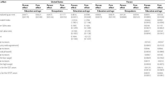
Table 6 Regressions of person and firm effects on economy-wide factors (with controls)

Firm effect United States France

Person effect Firm effect Person effect Firm effect Person effect Firm effect Person effect Firm effect Person effect Firm effect Person effect Firm effect

Education and age Occupations Education and age Education and age Occupations Education and age

Normalized quasi-rent 0.0471 (0.0170) 0.0623 (0.0180) 0.0475 (0.0126) 0.1177 (0.0192) 0.0816 (0.0251) 0.0780 (0.0269) 0.0003 (0.0073) 0.0678 (0.0139) 0.0128 (0.0088) 0.0594 (0.0123) 0.0093 (0.0085) 0.0536 (0.0128)

Herfindahl Index -2.3524

(1.9821) 2.2784 (2.1186) -0.0466 (0.0395) 0.0981 (0.0590)

Export-Sales ratio 0.1985

(0.1299) 0.1626 (0.1389) 0.0248 (0.0437) 0.1191 (0.0652)

Capital-Labor ratio -0.1903

(0.1055) -0.1295 (0.1128) 0.0037 (0.0094) 0.0169 (0.0141) Union 0.1484 (0.1344) -0.2125 (0.1437)

Wage increases -0.0165 -0.0347

(industry-wide agreement) (0.0083) (0.0123)

Wage increases 0.0046 0.0066

(individual-based) (0.0054) (0.0080)

Wage increases -0.0067 0.0185

(for the low-wage) (0.0069) (0.0102)

Wage increases 0.0019 -0.0232

(for the high-wage) (0.0050) (0.0075)

Votes for the CGT union -0.0129

(0.0314)

0.0616 (0.0469)

Votes for the CFDT union 0.0039

(0.0201)

IZA

Journal

o

fL

abor

Economics

2012,

1

:7

Page

20

of

25

Table 6 Regressions of person and firm effects on economy-wide factors (with controls)(Continued)

Votes for the FO union 0.0269

(0.0302)

-0.0631 (0.0451)

Votes for the CGC union 0.0343

(0.0179)

0.0507 (0.0267)

Union delegates -0.0037

(0.0050)

-0.0130 (0.0075)

Health and Security -0.0230 0.0111

Commissions (CHSCT) (0.0103) (0.0154)

R-Square 0.5255 0.8041 0.6114 0.6706 0.5583 0.8208 0.5905 0.5159 0.5076 0.6866 0.6406 0.7393

Number of Obs 70 70 70 70 66 66 95 95 95 95 93 93

structures changes the results quite markedly for the United States. In particular, the coef-ficient of the quasi-rent is divided by a factor of three in the firm effect regression. The other variables have little impact on the firm or the person effects in the presence of age and education controls. In particular, the product market variables appear to display little correlation with the person and firm effects, except for the capital-labor ratio which has a negative coefficient, potentially because of the substitution of capital for labor.

A first conclusion is that most of the person and firm effects in the United States are related to educational or occupational capital, specific to the industry. Much less is left for the quasi-rent to explain, even though its coefficients remain significant.

For France the estimates in Table 5 show that product market variables are strongly related to the firm effect. Furthermore, the number of agreements struck by unions directed at low-wage workers is positively related to the size of the firm effect. Indus-tries with few agreements targeted at the high-wage workers have relatively high firm effects. Individual-based agreements are positively associated with large person effects. The number of industry-wide agreements, which affect every worker in the industry, has a negative association with both person and firm effects in the industry–which may reflect the possibility that a compromise was negotiated taking many aspects of the industry into consideration or simply that the industry has many low-wage workers.

The institutional orientation of the union is also quite revealing. The CGT vote is related solely and positively to the firm effect. Interestingly, when the Herfindahl index, the capital-labor ratio, and the export to sales ratio of the industry are included, as shown in the last two columns, the CGT vote coefficient becomes insignificant. Therefore, the CGT appears to benefit from product market aspects of the industries in which this union is strong. The CFDT and, above all, the CGC are apparently strong among the more edu-cated workers, which translates their presence into larger person effects. Finally, a strong presence of union representatives, often present in low-wage manufacturing industries, translates into lower person effects.

In stark contrast with the United States, the results for France are little changed by the introduction of the education and age structure or occupations. For instance, the firm effect remains strongly related to the quasi-rent but not the person effect. Most interest-ingly, the strength of the relation between the product market variables and the firm effect is unchanged. Finally, the union variables have a similar effect on the firm component of the inter-industry differential but have, now, virtually no effect on the person component. The striking difference between the uncontrolled (Table 5) and controlled (Table 6) results for the U.S. and France, especially when the age and education structure variables are introduced, invites serious discussion of the reasons. The possibility that the weak industrial union presence in the U.S. vis-à-vis France permits far less mutual protection of the quasi-rents by the two sides and allows individual bargaining to distribute more of the firm effect to older or better educated workers. In France, where the industry-wide collective bargaining agreements permeate all sectors, there is simply much less scope for individual bargaining to target the quasi-rents.

More interestingly, and importantly, it is significantly related to the product market con-ditions prevailing in the industry. The person component of the differentials is mostly related to skills of the workforce, be it education or the lack thereof. In the United States, the person and the firm components of the inter-industry wage differentials appear to reflect some elements of bargaining and unionization, but they mostly reflect occupational or educational sorting across industries as well as capital specific to the industry.

8 Conclusion

We have specified and examined a model of long-term interindustry wage differences that decomposes the measure into a part due to unobservable individual heterogeneity and a part due to employer heterogeneity. We find that for both the United States and France this decomposition reveals much about the sources of the differences. A single aggregate measure, the quasi-rents per worker, accounts for a remarkably large percentage of the variation. It is more strongly related to the employer heterogeneity than to the individual heterogeneity, particularly in France where product market variables appear to play a sizeable role. Controls for the capital/labor ratio, product market concentration, and measurable demographic differences within sectors do not reduce the strength of this conclusion.

Predictably, the wage rate decomposition and the subsequent analysis of its components raise some new issues for labor economists. First, our analysis of these person and firm effects in relation to industry variables is not causal. It uses a model to provide interpreta-tion of observed correlainterpreta-tions. More is needed to go from correlainterpreta-tions to causality. Second, the fundamental decomposition is identifiable because longitudinally linked employer-employee data, whether sampled or from universes, provide a sufficiently rich description of the connectedness of the labor market. This connectedness, which we exploit to esti-mate the person and firm effects, can also be exploited to model the temporal variation in functions of these effects. In our present analysis, this temporal variation is entirely attributed to changes in the composition of the aggregates (industries) and not to changes in the structure of the compensation within aggregates (time-varying person and firm effects). Such a pursuit is one important extension of our work.

Endnotes

1_{Many technical details are elaborated in the Additional file 1: Online Appendix, available}

from theJournalor the authors.

2_{His argument is as follows. Note that, in the longitudinal data, lnw}a

it=lnE(wit|xit,i)= (xitβ+αi)+lnE

exp(ψJ(i,t)+εit|xit,i)Because the pure firm effectψJ(i,t)andεboth have

mean 0, and varianceσ_ψ2andσ_ε2respectively, we haveE[ exp(ψ+ε)]= expσ 2 ψ+σε2

2 ≈1,

assuming that bothψandεare normal, because, in the economy, the estimated values of σ_ψ2andσ_ε2are small (see Abowd et al. (2002a) and Abowd et al. 2002b) and because they can be taken as empirically independent of the person observed or unobserved character-istics. Hence,ψ_J(i,t)is a measure of the systematic premium paid to workeriby firm J(i,t) over her opportunity wage.

3_{The dominant employer is the one from whom the worker earned the most in the}

4_{This section is based upon the analysis in AKM, Abowd and Kramarz (1999a), and the}

handbook chapter (Abowd and Kramarz 1999b). The reader is referred to these papers for additional details.

5_{The Additional file 1: Appendix is available online from theJournaland the authors.}

6_{We are grateful to Thomas Lemieux for pointing this out to us.}

7_{This Additional file 1: Appendix is also available online from theJournalor the authors.}

8_{The labor market computations in this section were performed by the authors using the}

1986 and 1992 wage structure surveys.

9_{Similar results are also found using cross-sections of matched worker-firm data for the}

two countries (see Abowd et al. (2001)).

10_{See Peoples (1998) for a review of this literature in the United States. See Card (1986)}

for the airline industry; Black and Strahan (2001) for the banking industry.

11_{The Additional file 1: Appendix is available online from theJournalor the authors. See}

the notes to Additional file 1: Additional file 1: Appendix Tables A1 and A2 for additional information regarding the calculations.

12_{Note that the industry average person effect plus the industry average firm effect does}

not sum exactly to the industry average raw effect due to the fact that the models in the United States were estimated separately state-by-state then aggregated to the national level using weights representative of 1997 and a decomposition of the state-effect into a part due to state-average person effects, a part due to state-average firm effects, and an unexplained part (see ALM). For any given state, the decomposition is exact. For France the small discrepancy is due to the estimation of person and firm effects for all observa-tions and the presence of a small amount of missing industry data.

13_{The table displays summaries from two different correlation matrices. The first three}

rows are the correlation of French and American effects with each other weighted by the French industry employment. Hence the 3×3 block of correlations of the French mea-sures with themselves is symmetric but the 3×3 block of correlations of French measures with American measures is not. The correlation of American measures with themselves using French weights is not shown since it is not particularly interesting. Similarly the last three rows measure the correlations using American employment weights. Hence, the 3×3 block of correlations of American measures with themselves is symmetric but the correlation of American measures with French measures is not. Again, the correlation of French measures with themselves using American employment weights is not shown. 14_{The Additional file 1: Appendix B is available online from theJournaland the authors.}

15_{Two issues arise in the specification of equation (9). First, we note that measurement}

16_{We estimate the effects in Tables 5 and 6 using industry employment as the weight}

because we are interested in an equation that is representative of the entire economy, not one that is representative of a randomly selected industry.

Additional file

Additional file 1: Persistent Inter-Industry Wage Differences: Rent Sharing and Opportunity Costs (Online Appendix).

Competing interests

The IZA Journal of Labor Economics is committed to the IZA Guiding Principles of Research Integrity. The authors declare that they have observed these principles.

Acknowledgements

The authors gratefully acknowledge the assistance of Robert Creecy, U. S. Census Bureau, who developed the computational algorithms used in this paper. They also acknowledge funding from the NSF (SBER 9618111 to the NBER, and SES 9978093, 0339191, 0427889, and 1131848 to Cornell University). Joe Altonji, Orley Ashenfelter, Simon Burgess, David Card, Hank Farber, Hampton Finer, Juan Jimeno, Michael Krause, Michael Kremer, Julia Lane, Thomas Lemieux, David Margolis, Dale Mortensen, Walter Oi, Sébastien Perez-Duarte, Lars Vilhuber and seminar participants at many places provided valuable comments on earlier drafts. Melissa Bjelland, Benoit Dostie, Kaj Gittings, and Changhui Kang provided excellent research assistance. The French data used in this paper are confidential but the authors’ access is not exclusive. For further information contact Francis Kramarz. This document reports the results of research and analysis undertaken by the U.S. Census Bureau staff. It has undergone a Census Bureau review more limited in scope than that given to official Census Bureau publications. This document is released to inform interested parties of ongoing research and to encourage discussion of work in progress. This research is a part of the U.S. Census Bureau’s Longitudinal Employer-Household Dynamics Program (LEHD), which was partially supported by the National Science Foundation Grants SES-9978093, SES-0427889 to Cornell University (Cornell Institute for Social and Economic Research), the National Institute on Aging Grant R01 AG018854, and the Alfred P. Sloan Foundation. The views expressed herein are attributable only to the authors and do not represent the views of the U.S. Census Bureau, its program sponsors or data providers. Some of the data used in this paper are confidential from the LEHD Program. The Census Bureau supports researcher use of these data through the Research Data Centers (see: https://www.census.gov/ces/index.html).

Responsible Editor: V. Joseph Hotz

Author details

1_{School of Industrial and Labor Relations, Cornell University, US Census Bureau, CREST, IZA, and NBER, 261 Ives Hall,} Ithaca, NY 14853, USA.2_{CREST-ENSAE, CEPR, IZA, and IFAU, 15, boulevard Gabriel Péri, Malakoff, Cedex 92245, France.} 3_{Industrial Output Section, Federal Reserve Board of Governors, 20th Street and Constitution Avenue N.W., Washington,} D.C. 20551, USA.4_{LEHD, US Census Bureau, California Census Research Data Center, 4284 Public Affairs Building, UCLA,} Los Angeles, CA 90095, USA.5_{CREST-ENSAE, 15, boulevard Gabriel Péri, Malakoff, Cedex 92245, France.}

Received: 26 July 2012 Accepted: 22 August 2012 Published: 20 December 2012

References

Abowd J, Allain L (1996) Compensation structure and product market competition. Annales de l’économie et de statistique 41/42: 207–217

Abowd JM, Kramarz F (1999a) The analysis of labor markets using matched employer-employee data. In: Ashenfelter O Layard R (eds) Handbook of Labor Economics, Volume 3, Volume 3B, Chapter 40, pp. 2629–710, North Holland, Amsterdam

Abowd JM, Kramarz, F (1999b) Econometric analyses of linked employer–employee data. Labour Economics 6: 53–74 Abowd J, Lemieux T (1993) The effects of product market compettion on collective bargaining agreements: The case of

foreign competition in Canada. Q J Econ 108(4): 983–1014

Abowd JM, Finer H, Kramarz F (1999a) Individual and Firm Heterogeneity in Compensation: An analysis of matched longitudinal employer-employee data for the state of Washington. In: Haltiwanger J, Lane J, Theeuwes P (eds) The Creation and Analysis of Employer-Employee Matched Data, pp. 3–24. Elsevier-North Holland, Amsterdam Abowd JM, Kramarz F, Margolis DN (1999b) High wage workers and high wage firms. Econometrica 2: 251–334 Abowd JM, Kramarz F, Margolis DN, Troske KR (2001) The relative importance of employer and employee effects on

compensation: A comparison of France and the United States. J Jpn Int Economies 15(4): 419–436 Abowd JM, Creecy R, Kramarz F (2002a) Computing person and firm effects using linked longitudinal

employer-employee data. Technical Report TP2002-06, U.S. Census Bureau, LEHD Program

Abowd JM, Lengermann P, McKinney K (2002b) The measurement of human capital in the U.S economy. Technical Report TP 2002-09, U.S. Census Bureau LEHD Program

Abowd J, Kramarz F, Roux S (2006) Wages, mobility and firm performance: Advantages and insights from using matched worker-firm data. Econ J 116: F245–F285

Abowd JM, Stephens BE, Vilhuber L, Andersson F, McKinney KL, Roemer M, Woodcock SD (2009) The LEHD infrastructure files and the creation of the Quarterly Workforce Indicators. In: Dunne T, Jensen J, Roberts M (eds) Producer Dynamics: New Evidence from Micro Data, pp. 149–230. University of Chicago Press for the NBER

Bertrand M, Kramarz F (2002) Does entry regulatino hinder job creation?: Evidence from the french retail industry. Q J Economics 117(4): 1369–1414

Black S, Strahan P (2001) The division of spoils: Rent-sharing and discrimination in a deregulated industry. Am Econ Rev 91: 814–831

Brown C, Medoff J (1989) The employer size-wage effect. J Political Economy 97(5): 1027–1059

Cahuc P, Kramarz F (1997) Voice and loyalty as a delegation of authority: A model and a test on matched worker-firm data. J Labor Economics 15(4): 258–288

Cahuc P, Postel Vinay F, Robin J-M (2006) Wage bargaining with on-the-job search: Theory and evidence. Econometrica 74(2): 323–364

Card D (1986) Efficient contracts with costly adjustments: Short-run employment determination for airline mechanics. Am Econ Rev 76: 1045–1071

Card D, Heining J, Kline P (2012) Workplace heterogeneity and the rise of german wage inequality. Technical report, University of California-Berkeley

Dickens WT, Katz L (1987) Inter-industry wage differences and industry characteristics. In: Dickens, W T Leonard, J S (eds) Unemployment and the Structure of the Labor Market. Basil Blackwell, New York

Djankov S, Porta R, de Silanes FL, Schleifer A (2002) The regulation of entry. Q J Economics 1: 1–37

Farber H, Western B (2001) Accounting for the decline of unions in the private sector. J Labor Res 22: 459–486

Gibbons R, Katz L (1992) Does unmeasured ability explain inter-industry wage differentials? Rev Econ Studies 59: 515–535 Groshen E (1991) Souces of intra-industry wage dispersion: How much do employers matter? Q J Econ 106: 869–884 Goux D, Maurin É (1999) Persistence of interindustry wage differentials: A reexamination using matched worker-firm

panel data. J Labor Econ 17: 492–533

Haltiwanger J, Lane J, Theeuwes P (1999) The Creation and Analysis of Employer-Employee Matched Data. Elsevier-North Holland, Amsterdam

Kramarz F (2008) Offshoring, wages and employment: Evidence from data matching imports, firms and workers. Technical report, CREST. http://www.crest.fr/ckfinder/userfiles/files/Pageperso/kramarz/Offshoring072008.pdf cited on August 28, 2012

Kramarz F, Philippon T (2001) The impact of differntial payroll tax subsidies on minimum wage employment. J Public Econ 82: 115–146

Krueger A, Summers LH (1987) Reflections on the inter-industry wage structure. In: Lang K Leonard JS (eds) Unemployment and the Structure of Labor Markets. Basil Blackwell, Oxford

Krueger, A, Summers, L H (1988) Efficiency wages and the inter-industry wage structure. Econometrica 56(2): 259–293 Mortensen D (2003) Wage Dispersion: Why Are Similar Workers Paid Differently?. MIT Press, Cambridge, MA. ISBN

0262134330

Murphy KM, Topel RH (1987) Unemployment, risk, and earnings: Testing for equalizing wage differences in the labor market. In: Lang K, Leonard JS (eds) Unemployment and the Structure of Labor Markets. Basil Blackwell Peoples J (1998) Deregulation and the labor market. J Econ Perspect XII: 112–130

Postel-Vinay F, Robin J-M (2002) Wage dispersion with worker and employer heterogeneity. Econometrica 70: 2295–350 Shimer R (2005) The assignment of workers to jobs in an economy with coordination frictions. J Political Economy

113: 996–1025

doi:10.1186/2193-8997-1-7

Cite this article as:Abowdet al.:Persistent inter-industry wage differences: rent sharing and opportunity costs.IZA Journal of Labor Economics20121:7.

Submit your manuscript to a

journal and benefi t from:

7Convenient online submission 7Rigorous peer review

7Immediate publication on acceptance 7Open access: articles freely available online 7High visibility within the fi eld

7Retaining the copyright to your article