R E S E A R C H
Open Access
Fluχ
: a quality-driven dataflow model for data
intensive computing
S´ergio Esteves
*, Jo˜ao Nuno Silva and Lu´ıs Veiga
*Abstract
Today, there is a growing need for organizations to continuously analyze and process large waves of incoming data from the Internet. Such data processing schemes are often governed by complex dataflow systems, which are deployed atop highly-scalable infrastructures that need to manage data efficiently in order to enhance performance and alleviate costs.
Current workflow management systems enforce strict temporal synchronization among the various processing steps; however, this is not the most desirable functioning in a large number of scenarios. For example, considering dataflows that continuously analyze data upon the insertion/update of new entries in a data store, it would be wise to assess the level of modifications in data, before the trigger of the dataflow, that would minimize the number of executions (processing steps), reducing overhead and augmenting performance, while maintaining the dataflow processing results within certain coverage and freshness limit.
Towards this end, we introduce the notion of Quality-of-Data (QoD), which describes the level of modifications necessary on a data store to trigger processing steps, and thus conveying in the level of performance specified through data requirements. Also, this notion can be specially beneficial in cloud computing, where a dataflow computing service (SaaS) may provide certain QoD levels for different budgets.
In this article we proposeFluχ, a novel dataflow model, with framework and programming library support, for orchestrating data-based processing steps, over a NoSQL data store, whose triggering is based on the evaluation and dynamic enforcement of QoD constraints that are defined (and possibly adjusted automatically) for different sets of data. WithFluχwe demonstrate how dataflows can be leveraged to respond to quality boundaries that bring controlled and augmented performance, rationalization of resources, and task prioritization.
Keywords: Dataflow, Workflow, Quality-of-Data, Data store, NoSQL
1 Introduction
Current times have been witnessing an increase of massively scale web applications capable of handling extremely large data sets throughout the Internet. These data-intensive applications are owned by organizations, with cutting edge performance and scalability require-ments, whose success lies in the capability of analyzing and processing terabytes of incoming data feeds on a daily-basis. Such data processing computations are often governed by complex dataflows, since they allow bet-ter expressiveness and maintainability than low-level data processing (e.g., java map-reduce code).
*Correspondence: [email protected]; [email protected] Instituto Superior T´ecnico - UTL / INESC-ID Lisboa Distributed Systems Group Rua Alves Redol, 9, 1000-029 Lisboa, Portugal
Dataflows (or data processing workflows) can be rep-resented as directed acyclic graphs (DAGs) that express the dependencies between computations and data. These computations, or processing steps, can potentially be decoupled from object location, inter-object communica-tion, synchronization and scheduling; hence, being highly flexible on supporting parallel scalable and distributed computation. The data is either transferred directly from one processing step to another using intermediate files or via a shared storage system, such as a distributed file sys-tem or a database (which is our target in this particular work).
Another extensive use of dataflows has been for contin-uous and incremental processing. Here, vast amounts of raw data are continuously fed, as input, to cross an incre-mental processing pipeline in order to be transformed
into final structured and refined data. Examples include data aggregation in databases, web crawlers, data mining, and others from many different scientific domains, like sky surveys, forecasting, RNA-sequencing, or seismology [1-5].
The software infrastructure to setup, execute and mon-itor dataflows is commonly referred to as Workflow Man-agement System (WMS). Generally, WMSs either enforce strict temporal synchronization across the various input, intermediate and output data sets (i.e., following the SDF computing model [6]), or leave the temporal logic in the programmer hands, who have often to explicitly program non-synchronous behavior to meet application latency and prioritization requirements. For example, pro-cessing news documents faster than others in a web indexing system; or, in the astronomy domain, process-ing images, collected from ground-based telescopes, of objects that are closer to Earth first, and only then images that do not require immediate attention. Moreover, these systems do not account with the volume of data that arrives on each dataflow step, which could and should be used to reason about their performance impact on the system. Precisely, executing a processing step each time a small fragment of data arrives can have a great impact on performance, as opposed to executing only when a certain substantial quantity of new data is avail-able. Such issues are addressed in this work with a data quality-driven model based on the notion of what we call Quality-of-Data.
Informally, we define Quality-of-Data (QoD) as the abil-ity to provide different priorabil-ity to different data sets, users or dataflows, or to guarantee a certain level of perfor-mance of a dataflow. These guarantees can be enforced, for example, based on data size, number of hits in a certain data store object, or delay inclusion. High QoD should not be confused with high level of performance, but instead it conveys in the capability of strictly complying with QoD constraints defined over data sets.
With the QoD concept,a we are thus able to define and apply temporal semantics to dataflows based on the volume and importance of the data communicated between processing steps. Moreover, relying on QoD we can augment the throughput of the dataflow and reduce the number of its executions while keeping the results within acceptable limits. Also, this concept is particu-larly interesting in (public) cloud computing, where a dataflow service (SaaS) may provide different QoD lev-els for different budgets. Therefore, this work can also give a contribute to the new studies addressing the cost and performance of deploying dataflows in the cloud (e.g., [7]).
Given the current envisagement, we propose a novel dataflow model, with framework and programming library support, for orchestrating data-based computation
stages (actions), over a NoSQL data store, whose trigger-ing is based on the evaluation and dynamic enforcement of QoD constraints that are defined, and possibly adjusted automatically, for different sets of data. With this frame-work, named Fluχ, we enable the setup of dataflows whose execution is guided and controlled to comply with certain QoD requirements, delivering thus: controlled performance (i.e., improved or degraded); rationaliza-tion of resource usage; execurationaliza-tion prioritizarationaliza-tion based on relative importance of data; and augmented throughput between processing steps.
We implementedFluχusing an existing WMS, that was adapted to enforce our model and triggering semantics, and adopted, as the underlying data store, the HBase tab-ular storage [8]. Our results show thatFluχ is able to: i) ensure result convergence, hence showing that the QoD model does not introduce significant errors, ii) save signif-icant computational resources by avoiding wasteful repet-itive execution of dataflow steps, and iii) consequently, reduce machine load and improve resource efficiency, in cluster and cloud infrastructures, for equivalent levels of data valueprovided to, and as perceived by, decision makers.
Shortcomings of state-of-the-art solutions include (to the best of our knowledge): i) lack of tools to enable trans-parent asynchronous behavior in workflow systems; ii) no support for dataflows to share data through highly-scalable cloud-like databases; iii) lack of integration, in mostly loosely-coupled environments, between the work-flow management and the underlying intermediate data (which is seen as opaque); and iv) no quality of service, and of data, is enforced (at least in a flexible manner).
The remainder of this article is organized as follows. Section 2 presents the Fluχ dataflow model based on the QoD notion. Section 3 describes an archetypal meta-architecture of the Fluχ middleware framework, and Section 4 offers its relevant implementation aspects. Then, Section 5 presents a performance evaluation, and Section 6 reviews related work. Finally, we draw all appro-priate conclusions in Section 7.
2 Abstract dataflow model
Our dataflow model can be expressed as a directed acyclic graph (DAG), where each node represents a pro-cessing step (designated here byaction) that must perform changes in a data store; and the edges between actions represent dependencies, meaning that an action needs the output of another action to get executed (naturally, these dependencies need to be decoupled from WMS implementation so that the same actions can be com-bined in different ways). More precisely, each actionA, in a dataflowD, is executed only after all actionsA’preceding A(denotedA≺DA) inDhave been executed at least once
(elaborated hereafter). In addition, actions can be divided in: input actions, which are supplied with data from exter-nal sources; intermediate actions, which receive data from other actions; and output actions, whose generated data is read by external consumers.
Unlike the other typical models, our approach takes a step further: the end of execution of a nodeAdoes not mean that the successor nodesA’(denotedADA), that
depend onA, will be immediately triggered (like it usually happens). Instead, successor nodes should be triggered as soon as A has finished its execution and has also per-formed a sufficient level of changes in the data store that comply with certain QoD requirements (which can cause a node being executed multiple times with the successor nodes being triggered only once). If such changes do not occur in a given time frame, successor nodes would even-tually be triggered. Hence, the QoD requirements evaluate the volume of data input fed to an action that is worth its execution. This is the key difference and novelty of our approach that breaks through the SDF (synchronous data-flow) computing model.
The amount of data changes (QoD) necessary to trig-ger an action, denoted by κ, is specified using multi-dimensional vectors that associate QoD constraints with data object containers, such as a column or group of columns in a table of a given column-oriented database.κ
bounds the maximum level of changes through numeric scalar vectors defined for each of the following orthogonal dimensions: time (θ), sequence (σ), and value (ν).
TimeSpecifies the maximum time an action can be on hold (without being triggered) since its last execution occurred. Consideringθ (o)provides the time (e.g., seconds) passed since the last execution of a certain action that is dependent on the availability of data in the object containero, this time constraintκθ
enforces thatθ (o) < κθat any given time.
SequenceSpecifies the number of still unapplied updates to an object container object containero upon which, the action that depends ono is triggered. Consideringσ (o)indicates the number of applied updates overo, this sequence constraintκσenforces
thatσ (o) < κσ at any given time.
ValueSpecifies the maximum relative divergence between the updated state of an object containero and its initial state, or against a constant (e.g., top value), since the last execution of an action dependent ono. Consideringν(o)provides that difference (e.g., in percentage), this value constraintκν enforces that
ν(o) < κνat any given time. It captures the impact or
importance of updates in the last state.
These constraints are used to trigger the execution of actions. When they are reached, the action is executed (or scheduled to be executed). Access to the object contain-ers is not blocked but update countcontain-ers are still maintained in synch. Only if specified (and it is not required for the intended applications in this paper), will the constraints, when reached, block access to the data containers, pre-venting further updates until the action is re-executed.
The QoD boundκ, associated with an object container o, is reached when any of its vectors has been reached, i.e.,θ (o) ≥ κθ ∨σ (o) ≥ κσ ∨ν(o) ≥ κν. Also, grouped containers (e.g., a column and a row) are treated as single containers, in the sense that modifications performed on any of the grouped objects change the sameκ.
Moreover, the triggering of an action can depend on the updates performed on multiple database object con-tainers, each of which possibly associated with a different
κ. Hence, it is necessary to combine all associated con-straints to produce a single binary outcome, deciding whether or not the action should be triggered. To address this, we provide a QoD specification algebra with the two logical operatorsandandor(∧and∨) that can be used between any pair of QoD bounds. Theand opera-tor requires that every associated QoD boundκ should be reached in order to trigger an associated action; while theorrequires that at least oneκ should be reached for the triggering of the action. Following the classical seman-tics, the operatorandhas precedence over operatoror. For example, an actionAcan be associated with the expres-sionκ1∨κ2∧κ3, which causes the triggering ofAwhenκ1
is reached, orκ2andκ3have been both reached.
Furthermore, we also allow a unique definition for the combination of allκbounds, instead of individually spec-ifying operators for every pair of bounds. The pre-built available definitions are:
all(∀) An action is triggerediff all associatedκ bounds are reached.
at-least-one(∃1) An action is triggered iff at least on associatedκis reached.
majority((n+1)/2) An action is triggered iff the majority of associatedκ bounds are reached (e.g., 2 of 3 bounds, or 3 of 4 bounds, are reached).
2.1 Prototypical example
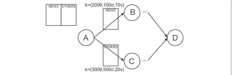
Figure 1 depicts a simple and partial example dataflow of a typical web crawler, which serves as motivation and familiar prototypical example to introduce dataflows. StepA crawls documents over the web and stores their text on stable storage, either in a file system or as an opaque object in a database (e.g., no-SQL), along with some metadata extracted from the document contents, HTTP response headers, or derived from some prepro-cessing based on title words, URL, or tags. Depending on the class of the accessed pages, their content is stored in different tables: one for the news items, other for the remaining static pages.
Steps B and C are similar in function, in the sense that they process existing documents, generating word counts of the words present in the document, along with the URL containing them. The difference being that step B processes specifically only those documents identi-fied or marked as containing news-related content in the previous step.
Since news pages change more frequency and are more relevant,Bhas stricter QoD requirements, and therefore is processed faster (i.e., activated more often). Its diver-gence bounds are lower, meaning that it will take less time (200 vs 300 seconds), fewer new documents crawled (100 vs 500), and/or fewer modifications on new versions of crawled documents (10% vs 20% of contents), in order to activate it.
Finally, in stepD, all the information generated by the previous executions of steps B andC is joined and the inverted index (word→ {list of URLs}, for each word) is generated.
This whole process could be performed resorting to Map-Reduce programs but, as we describe in Section 6, since Map-Reduce programs are becoming increasingly larger and more complex, their reuse can be leveraged chaining them into workflows, reducing development
effort. In Section 5 we will address a more elaborate example.
3 Architecture
In this section we present the architecture and design choices of theFluχ middleware framework that is capa-ble of managing dataflows following the model described in the previous section (Section 2). The Fluχ frame-work, is designed to be tightly coupled with a large-scale (NoSQL) data store, enabling the construction of quality-driven dataflows in which the triggering of processing steps (actions) may be delayed, but still complying with QoD requirements defined over the stored data.
This framework may be particularly useful in public cloud platforms where it can be offered as a Software-as-a-Service (SaaS) in which the QoD requirements are defined according to certain budgets; i.e., small budgets would have stricter QoD constraints, and large budgets looser QoD constraints.
Figure 2 shows a distributed network architecture in the cloud whereby a dataflow is set up to be executed upon a cluster of machines connected through a local network. More precisely, a coordinator machine, run-ning a WMS withFluχ, allocates the dataflow actions to available worker nodes and the input/output data is com-municated between actions via a shared cloud tabular data store. In this particular work we abstract from the details of scheduling and running actions in parallel; our focus here is that actions share input, intermediate, and out-put data through a distributed cloud database (instead of intermediate files, like it usually happens).
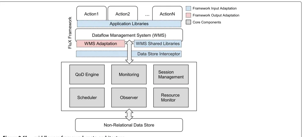
Figure 3 depicts an archetypal meta-architecture of the Fluχ middleware framework, which operates in the middle of a dataflow manager and an underlying non-relational tabular storage. Actions of a dataflow run on top of the dataflow manager and they must share data through the underlying storage. These actions may consist
Figure 2Network architecture.
of Java applications, scripts expressed through high-level languages for data analysis (e.g., Apache Pig [9]), map-reduce jobs, as well as other out-of-the-box solutions. The components outlined with no solid line dash are optional meta-components for the adaptation ofFluχ.
The framework can operate either with its own pro-vided simple WMS, or with an existing dataflow manager by means of the WMS Adaptation Component (colored in red). This inherent dependency of our framework with a WMS concerns mainly to the triggering notifications. With our WMS, we simply use a provided API through whichFluχ signals the triggering of actions. While using an existing WMS, we need to change its source and pro-vide an adaptation component that controls the triggering of actions upon request.
Since Fluχ needs to be aware of the data modifica-tions performed by acmodifica-tions in the underlying database, we contemplate three different solutions, regarding the adaptation of database libraries, that can be derived from the meta-architecture. The components colored in gray within the middleware are the core components and should be included by every derived solution; and the components colored in blue represent the three different alternatives for the adaptation, which are described as follows.
Application LibrariesThis solution consists of adapting application libraries, referenced in actions, that are used to interact directly with the data store via its client API. It is a bit intrusive in the sense that applications need to be modified, albeit we intend to provide tools so that this process may be completely automatized.
WMS Shared LibrariesThis alternative is on a lower layer and works for actions that need to access the database through WMS shared libraries (e.g., pig scripts or any other high-level language that must be compiled by the WMS). It provides transparency to actions, that do not need to be modified to work with
Fluχ.
Data Store InterceptorThis solution functions as a proxy that implements the underlying database communication protocol and intercepts the calls from the applications or WMS directed to the database; hence, achieving full transparency
regarding action code. Applications may only interact with the data store via this proxy, and therefore they should define as the database entry-point the address of the proxy (probably in the form of URL).
Next, we describe the responsibilities and purpose of each of the components present in theFluχframework. MonitoringThis component analyzes all requests
directed to the database. It uses information about update requests to maintain the current state of control data regarding the quality-of-data; and also collects statistics regarding access patterns to stored data (mainly read operations) in order to
automatically adjust the QoD levels, in the view of the improvement of the overall system
performance.
Session ManagementIt manages the configurations of the QoD constraints, over data objects, through the meta-data that is provided, along with the dataflow specification, and defined for each different dataflow. A dataflow specification is then derived to the target WMS.
QoD EngineIt maintains data structures and control meta-data which are used to evaluate and decide when to trigger next actions, obeying to QoD specifications.
SchedulerThis component verifies the time constraints over the data. When the time for triggering of successor actions expires, the Scheduler notifies the QoD Engine component in order to clear the associated QoD state and notify the WMS to execute the next processing steps.
ObserverIt provides mechanisms to scan the data store for modifications in case the updates performed do not go through the Monitoring component.
Resource MonitorThis component is responsible for monitoring the resource utilization and load of the machines allocated to execute dataflows. It informs the QoD Engine about the computation loads at runtime in order to automatically tune the QoD constraints.
3.1 Session management, metadata and dataflow isolation
Dataflow specification schemas need to be provided to register dataflows with theFluχframework. They should contain the description of the dataflow graph where each action must explicitly specify the underlying database object containers (e.g., table, column, or row) it depends and the relative QoD requirements necessary to the action triggering. Precisely, one QoD bound,κ, can be provided either for single database containers associated or for groups of object containers (e.g., several columns cov-ered by the sameκ); these two ways of associateκ imply different QoD evaluation and enforcement.
QoD constraints (time, sequence, and value) can be specified as either single values or intervals of values. The former guarantees always the same quality degree, while the latter is used for dynamic adjustment at runtime: each interval relies on two numerical scalars that are used for specifying the minimum and maximum QoD bounds respectively, and the QoD Engine component adjusts κ
within the interval as needed. If no bound is associ-ated with an actionA, then it is assumed thatAshould be triggered right after the execution of its precedent actions (i.e., strict temporal synchronism). After dataflow registration, the underlying database schema is extended to incorporate the metadata related with the QoD bound and QoD control state. Specifically, it is necessary to have maps that given a dataflow, an action node, and a database object container, return the quality bound and current state.
It may happen that database object containers, asso-ciated with actions of a certain dataflow, can be being written by other dataflows or external applications (and thus changing the triggering semantics). To disentangle such conflicts, we consider three isolation modes through which our framework can be configured:
Normal ModeIt relies on an optimistic approach in which it is assumed that nothing changes the database containers besides the dataflows. In this case, different dataflows will share the same QoD state; i.e., whenever data is changed on a DBMS object
container, the QoD state of all actions associated with that object are changed irrespective of which active dataflow has caused the modifications.
Observer ModeThis (pessimistic) mode assumes that dataflows are not the only entities performing changes on database objects. Therefore, it resorts to observers to scan the objects to detect modifications, since it is not guaranteed that every update passes through the Monitoring component.
external processes are also writing to the same DBMS objects. This mode implies the creation of a notify column (described hereafter) per each dataflow.
Since database object containers are likely to receive a vast volume of data items (e.g., a column with millions of keys being written), it could be very inefficient for observers to scan the whole columns and find those that have been changed. Therefore, we resort to a notifica-tion mechanism where each updated item in a container needs to write an entry in an auxiliary data structure. For example, every key written in a certain column would have to also write a timestamp in a special column (notify column); and, thus, the scans will only cover that notify column, which is much more efficient in a column-oriented NoSQL data store.
3.2 Evaluation and enforcement of quality-of-data bounds
The QoD state of a database object containero, for an action A, is updated every time an update is perceived by Fluχ through the Monitoring and Observer compo-nents. Upon such event, it is necessary to identify the actionAthat made the update (A ≺A) and the affected object container,o, which is sent by the client libraries; this, in order to retrieve the quality bound and current state associated through the metadata. Then, givenAand o, we can find all successor actions ofA, includingA, that are dependent on the updates performed ono, and thus update their QoD state (i.e., the state of each successor action depending ono). Specifically, we need to increment all of the associated vectorsσ and re-compute the ratio modified keys/total keys, hold in allνvectors. Afterwards, the QoD state of a pair (action, object) needs to be com-pared against its relative QoD reference bound (i.e., the maximum level of changes allowed,κ).
The evaluation of the quality vectorsσandν, to decide if an actionAshould be triggered or not, may take place at one of the following times: a) every time a write opera-tion is performed by a precedent acopera-tion ofA; b) every time a precedent action finishes completely its execution; or c) periodically between a given time frame. These options can be combined together; e.g., it might be of use to com-bine option c) with a) or b), for the case where precedent actions ofAtake very long periods of time in performing computations and generating output. Despite option a) being the most accurate, it is the least efficient, especially when dealing with large bursts of updates.
To evaluate the time constraint,θ,Fluχ uses timers to check periodically (e.g., every second) if there is any times-tamp inθabout to expire (i.e., a QoD bound that is almost reached). Specifically, references to actions are held in a list ordered ascending by time of expiration, which is
the time of last execution of a dependent action plusθ. In effect, the Scheduler component starts from the first element of the list checking if timestamps are older or equal than current time. As the list is ordered, the Sched-uler has only to fail one check to ignore the rest of the list; e.g., if the check on the first element fails (its timestamp has not expired yet), the Scheduler does not need to check the remaining elements of the list.
As described in Section 2, the possible various QoD states, associated with an action, can be combined using provided operators. If no operators or mode are provided, the modeall is used, enforcing that every single associ-ated QoD bound should be reached in order to trigger the relative action. If any limit is reached and an action is initi-ated, all QoD state vectors associated with that action are reset:θreceives a new timestamp,σandνgo to zero. 3.3 Dynamic adjustment of quality-of-data constraints As previously mentioned, users may also specify intervals of values on the QoD vectors (instead of single values), and let the framework automatically adjust the quality con-straints (within the intervals), hence varying the level of data modifications necessary to trigger successor actions, while preventing excessive load and error accumulation. This adjustment, performed by the QoD Engine compo-nent, is driven by two factors: i) the frequency of recent write operations to data items, during a given time frame; and ii) the current availability of computer resources and relative capabilities.
As for the former factor, we relax the QoD bound upon many consecutive updates, in an attempt to reduce the inherent overhead of triggering a given action an excessive number of times; i.e., we try to feed an action with as much data as possible within the upper boundary, as we antic-ipate further new input, instead of triggering that action with smaller subsets of that same data; hence, increas-ing throughput and resource efficiency. Conversely, we restrict the bound when updates are becoming less fre-quent and more spaced in time to increase the speed and reduce latency of the pipeline and dataflow processing steps.
These two factors can be entwined in the following way. Assuming the outcome of the assessment of each factor is either:restrict,relax, ornone; if one factor decidesrelax and the other decidesrestrict, then no action is taken (i.e., factors disagree). If one factor decidesrelaxorrestrictand the other decidesnone, then the resulting bound isrelaxed orrestrictedrespectively. Otherwise, the factors agree and the adjustment is made in accordance with the outcome (relax,restrict, ornone).
For not-so-expert users, we also provide a mechanism to automatically and dynamically adjust the QoD con-straints. Users have only to specify thesignificance factor, i.e., the percentage of changes in the dataflow output (or against a reference) that would be meaningful and signif-icant to decision-makers. For example, an air-sampling smoke detector should only issue a signal to a fire alarm system if the concentration of micro particles of combus-tion found is high enough (or significant); e.g., the fire alarm should not be triggered by the smoke of a simple cigar.
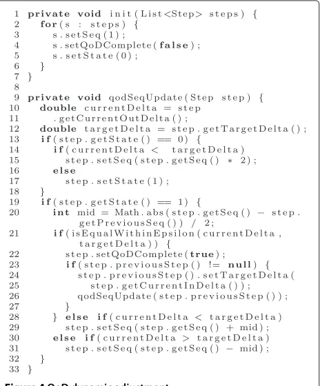
In this mode, vector elementθ is simply set to a default constant. Figure 4 shows how the sequence constraint (σ) is adjusted, by successive approximation and assessment, ensuring that the target significance is met at the out-put of the final step. This, by inferring, backwards along the dataflow, the maximum QoD at each step that still achieves it.
Figure 4QoD dynamic adjustment.
First, theσconstraint in all steps, besides the first, is ini-tialized to 1, meaning that every time a step completes its execution, performing at least 1 update, all its successors are triggered (like in the SDF model). TheqodSeqUpdate method is called upon a wave of incoming data over the steps that have not been adjusted yet (checked through theqodCompleteboolean). First (lines 13-18),σis doubled until the amount of variation in the output (currentDelta) goes above the significance factor (targetDelta). This vari-ation is calculated by summing the differences (in absolute value) between current and previous row’s values and dividing by the sum of all previous values. The goal is to makecurrentDeltaandtargetDeltato match or be within a given smallε(methodisEqualWithinEpsilon).
After this first stage to find the maximum, σ starts to converge to the optimal value, thereby decreasing its value whencurrentDeltais greater thantargetDelta, and increasing when it is lower (lines 28-31). If they match (lines 21-27) - in reality within a givenε, the optimal value of σ was found, and the qodSeqUpdateis called recur-sively for the predecessor step (if any), thereby setting its targetDeltato thecurrentInDelta(i.e., the current amount of variation in the input of the current step).
Applying this mechanism to the σ constraint is suffi-cient for dataflows where output variation across waves is mostly stable (not necessarily linearly dependent), given the number of updates to the input. When this rela-tionship does not hold, the dynamic adjustment mecha-nism targets theνconstraint instead, using an analogous approach to Figure 4. This way, it attempts to deter-mine the maximum magnitude of the modifications made at the input of each step, regardless of the actual num-ber of updates, that would still not produce any rele-vant change in the significance of the dataflow output results.
4 Implementation
In this section we present the relevant implementation details of a developed prototype, as a proof of concept, with the architecture aforementioned to demonstrate the advantages of our dataflow model when deployed as a WMS for high-performance and large-scale data stores.
4.1 Adopted technology
of a certain action; naturally, these notifications share the same action identifiers.
As for the lower layer, and although the framework can be adapted to work with other non-relational data stores, in the scope of this particular work, our target is BigTable [12] open-source Java clone, HBase [8], which we used as an instance of the underlying storage. This database system is a sparse, multi-dimensional sorted map, indexed by row, column (includes family and qual-ifier), and timestamp; the mapped values are simply an uninterpreted array of bytes. It is column-oriented, mean-ing that most queries only involve a few columns in a wide range, thus significantly reducing I/O. Moreover, these databases scale to billions of rows and millions of columns, while ensuring that write and read performance remain constant.
Finally, Fluχ was also built in Java, and uses, i.a., the Saxon http://saxon.sourceforge.net/ XPath engine to read and process XML configurations files (e.g., the dataflow description); and the SIGAR http://support.hyperic.com/ display/SIGAR/Home library for monitoring resource usage and machine loads. For efficiency, we followed the solution of adapting the HBase client libraries used by Java classes, representing the type of actions we tried at evaluation stage.
4.2 Library support and API
In order to intercept the updates performed by actions, we adapted the HBase client libraries by extending the implementation of some of their classes while maintain-ing their original APIs. http://hbase.apache.org/apidocs/ overview-summary.html Namely, the implementation of the classes Configuration.java, HBaseConfiguration.java, andHTable.java, were modified to intercept every update performed on HBase, especiallyputanddeleteoperations, and send the needed parameters (like action, operation, table, and column identifiers) to theFluχframework.
Applications need therefore only to be slightly modified to use our API. Specifically, only the import declarations of the HBase packages need to be changed toFluχ pack-ages, since our API is practically the same. To ease such process, we provide tools that automatically modify all the necessary import declarations, thereby patching the java bytecode at loading time.
4.3 Definition of dataflows with QoD bounds
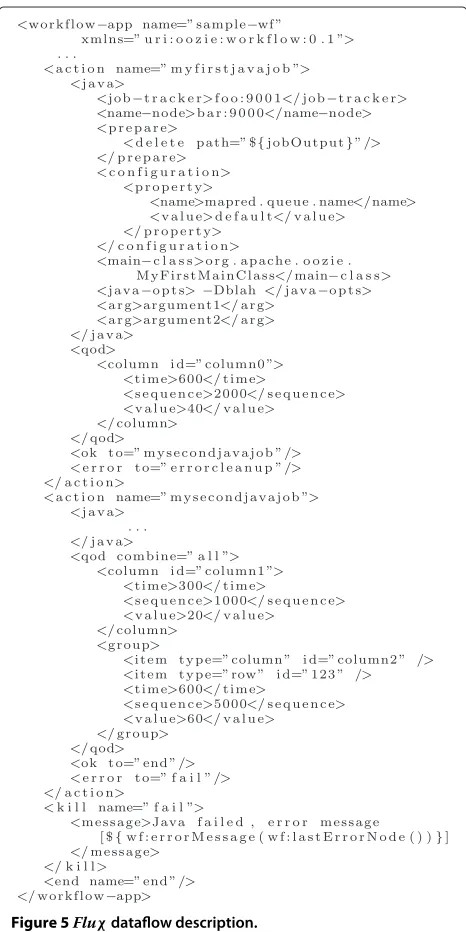
The QoD constraints, referring to the maximum degree of data modifications, are specified along with standard Oozie XML schemas (version 0.2), and given to the Fluχmiddleware with an associated dataflow description. Specifically, we introduced in the respective XSD the new elementqod, which can be used inside the elementaction. Insideqod, it is necessary to indicate the data object con-tainers associated, i.e., using the elementstable,column,
row, or group. Each of these elements must specify the three constraints time (a decimal indicating the number of seconds), sequence (an integer), and value (an integer indicating the percentage of modifications), that are com-bined through the method defined in the qod attribute combine. Additionally, the elementgroup groups object containers, which are specified through the elementitem, that should be handled at the same QoD degree. Next, we present an example, in Figure 5, omitting some details for readability purposes.
These particular dataflow descriptions are then auto-matically adapted to the regular Oozie schema (i.e., with-out the QoD elements) and fed to the Oozie manager.
Hence, our framework controls the upper workflow man-agement system and it is not necessary to perform addi-tional configurations on such external systems (i.e., all configurations must go throughFluχ). Nevertheless, we envision in the future for a more general dataflow descrip-tion, where it can be, afterwards, automatically adapted to a range of popular WMSs.
5 Evaluation
This section presents the evaluation of theFluχ frame-work and its benefits when compared with the regular DAG semantics (i.e., SDF with no QoD enforcement). More precisely, and attending to our objectives, we ana-lyze the gains ofFluχ with dataflows for continuous and incremental processing in terms of: i) result convergence, as the dataflow execution pipeline advances; ii) error cov-erage; and iii) machine loads and resource usage through the amount of executions performed/saved. All tests were conducted using 6 machines with an Intel Core i7-2600K CPU at 3.40GHz, 11926MB of available RAM memory, and HDD 7200RPM SATA 6Gb/s 32MB cache, connected by 1 Gigabit LAN.
5.1 Prototypical scenario
For evaluating our model and framework we relied on a dataflow, for continuous and incremental processing, that expresses a simulation of a prototypical scenario inspired by the calculation the Air Quality Health Index (AQHI), www.ec.gc.ca/cas-aqhi/ used in Canada. It captures the potential human health risk from air pollution in a cer-tain geographic area, typically a city, while allowing for more localized information. More specifically, the incom-ing data fed to this dataflow is obtained through several detectors equally distributed over an area of 10000 square units. Each detector comprises three sensors to gauge the amount of Ozone (O3), Particulate Matter (PM2.5) and Nitrogen Dioxide (NO2). In effect, each sensor cor-responds to a different generating function, following a distribution with smooth variations across space (i.e., real-istic while exactness not relevant for our purposes), which
will provide the necessary data to the dataflow. These gen-erating functions return a value from 0 to 100, where 0 and 100 are, respectively, the minimum and maximum known values of O3, PM2.5 or NO2. At the end, in the final step of the dataflow, the index is generated, thereby producing a number that is mapped into a class of health risk: low (1-3), moderate (4-6), high (7-10), and very high (above 10).
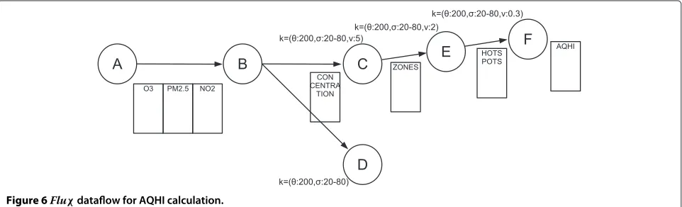
Figure 6 illustrates the dataflow with the associated QoD vectors and the main HBase columns (some columns were omitted for readability purposes) that comprise the object containers in which the processing steps’ triggering depends on.kspecifies i) the maximum time, in seconds, the action can be on hold; ii) the minimum amount, in percentage, of changes necessary to the triggering (e.g., 20% associated to stepC means that this action will be triggered when at least 20% of the detectors have been changed by stepB; and iii) the maximum accepted diver-gence, in units.
We describe each processing step in the following.
Step A:This step continuously feeds data to the dataflow by reading sensors from detectors that perceive changes in the atmosphere (i.e., randomly chosen in practice) to simulate asynchronous and deferred arrival of update sensory data. The values from each sensor are written in three columns (each row is a different detector) which are grouped as a single object container with one associatedk.
Step B:Calculates the combined concentration (of pollution) of the three sensors for each detector whose values were changed in the previous step. Every single calculated value (a number from 0 to 100 also) is written on columnconcentration.
Step C:Processes the concentrations of small areas, called zones, encircled by the previously changed detectors. These zones can be seen as small squares within the overall considered area and comprise the adjacent detectors (until a distance of two in every direction). The concentration of a zone is given by a simple
multiplicative model of the concentration of each comprising detector.
Step D:Calculates the concentration of points of the city between detectors, thereby averaging the
concentration perceived by surrounding detectors; and plots a chart containing a representation of the concentrations throughout the whole probed area, for displaying purposes, and reference of
concentration and air quality risk indicator in localized areas of a city (as traditionally, red and darker means higher risk, while green and lighter yellow means reduced risk). This step can be executed in parallel with Step E.
Step E:Analyzes the previous stored zones and respective concentrations in order to detect hotspots; i.e., zones where the overall concentration is above a certain reference. Zones deemed as hotspots are stored in columnhotspots for further analyzation.
Step F:Performs final reasoning about the hotspots detected, thereby combining, through a simple additive model, the amount (in percentage) of hotspots identified with the average concentration of pollution (O3,PM2.5andNO2) on all hotspots. Then,
the AQHI index is produced and stored for each wave of incoming data.
We conducted the evaluation for 2500 (50×50) to 40000 (200× 200) detectors with 1 to 6 nodes and averaged the results over several runs to reduce noise. We simu-lated this experiment as though we were analyzing the pollution of a city for a week, with a wave of incoming data (from changed detectors) fed to the dataflow at each hour, which performs 168 waves in total (24 hours per 7 days). Also, we used distributions of pollution with 3 dif-ferent tendencies in the generating functions (mimicking the sensors): increasing over time, decreasing over time, and globally uniform over time. Following, we analyze the
most important aspects of correctness and performance, for all the steps with QoD enforcement in the AQHI dataflow.
5.2 Step C analysis
Through Figure 7 we may see the pollution concentra-tion, on average of all zones, per each wave, while varying the QoD sequence vector, σ, in 20, 40, 60 and 80% of changed detectors (new data), and comparing against the concentration without using QoD. As depicted, the zone concentration on average with QoD converges to the con-centration without QoD. It takes more time (or waves) to converge as we increase the minimum percentage of detectors detecting changes (σ). In this particular trial, the tendency configured on the generating functions was to increase the pollution as the number of waves increase. Our trials allow us to show that the differences between values calculated with and without QoD are always repre-sentatively small and bounded. Moreover, our other trials also show that the values of concentration with and with-out QoD mostly converge, i.e. differences are diminishing. This confirms the initial motivation that it would waste resources, for most purposes, to execute the dataflow completely for each wave, as the increase in output accu-racy may be deemed as not significant, or relevant.
Figure 8 shows the maximum deviation (or error) of the concentration calculated, in relation to the pollu-tion observed with no QoD, when varying σ from 10 to 100%, meaning triggering execution only when there is new input for all sensors. The maximum error always stays below our defined threshold (vectorν) and the error increases with a linearly tendency as the waves or number of changed detectors increase. Despite, some noise and jit-ters (introduced by the variation of hundreds or thousands of sensors), the linear trend is clearly observable.
Through Figure 9 we can see that the number of exe-cutions decreases in an almost linear fashion as the
Figure 8Zone concentration maximum error with increasing QoD boundsσ.
allowed percentage of changed detectors (σ) increases. The number of step executions performed without QoD is naturally equal to the number of waves, 168, correspond-ing to the 100%. Whenσwas 25% we saved about 20% of 168 executions (i.e., fewer 33 executions than using regu-lar DAG semantics); and for 80% of detected changes we only performed 80 executions (48%). The machine loads and resource utilization were naturally proportional to the savings presented here.
5.3 Step D analysis
We present the graphs generated during a day (24 sam-ples) using regular DAG semantics and contrast them against theFluχmodel with QoD, for 20, 40, 60 and 80% of variation in vectorσ.
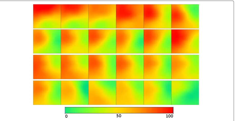
Without QoD, Figure 10 illustrates the evolution of the concentration of pollution in the city during a day. Areas colored in shades of green represent safer zones with lower pollution concentrations (low health risk);
yellow areas represent medium pollution concentration (moderate health risk); and colors ranging from orange to red indicate hotspots (high and very high health risk).
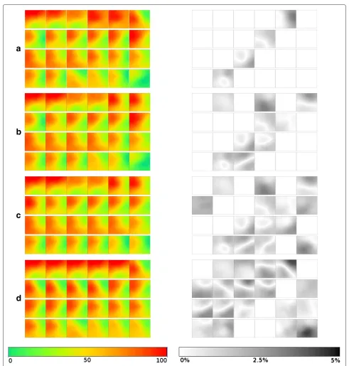
Figure 11 presents a similar matrix on the left and a difference matrix on the right. The former illustrates the evolution of pollution, but enforcing QoD, which means that not all 24 samples are generated, and thus there are repeated samples (i.e., during 2 or more hours the samples can be equal). The latter shows the differences between the repeated samples and the original ones (generated for each hour without QoD) with a maximum error of 5%, representing the darkest areas. Hence, brighter areas mean that the differences were minimal.
Figure 11a depicts a matrix with tiles generated when 20% of detectors have perceived changes. The divergence was minimal: only the 5th not-updated tile was darker (above 2.5% of difference) as at that hour the pollution had already decreased.
Figure 10Samples collected during 24 hours with no QoD enforcement.
In Figure 11b, 40% of changed detectors are needed in order to generate new and updated tiles. The black and white matrix shows slightly darker tiles than the previ-ous trial (Figure 11a) for the first hours of the day. Again, the levels of pollution at that hour were decreasing. When dealing with the opposite situation, levels increasing, the vectorν component comes to place and guarantees that a strong variation on pollution (above 5%) concentrations will cause the graph to be re-generated.
Through Figure 11c we can see that the generated tiles follow the same tendency of becoming darker asσ aug-ments. The difference matrix shows moderate variations in the tiles per hour, however notice that more than a half of the detectors have perceived changes (this hints that it might not be the most appropriate value ofσ for a real environment).
Finally, with aσ of 80% (Figure 11d) more error was introduced, but still within the acceptable limit of 5%. The contiguous black and white tiles do not show much dif-ference in their color, but, instead, on the location of the pollution concentrations; meaning that there is not much variation in the overall concentration levels of pollution and that the pollution is flowing from area to area.
To conclude, we can see that for higher levels of changed detectors (60 and 80%) the differences and errors are higher, but this higher divergence on some tiles happened due to the levels of pollution being greater with QoD than with the original tiles calculated without QoD (and not the opposite, which would be more dangerous). Notwith-standing, black and white graphs in general were brighter
and thus acceptable (especially for realistic and lower levels ofσ), supporting the intuitive notion and our argu-ments that the dataflow does not need to be recalculated every time a single, or a few, changes occur.
5.4 Step E analysis
Now using uniform distributions to generate the pollu-tion concentrapollu-tions, we may observe, through the charts of Figure 12, that the most divergence of concentration in hotspots, between using QoD and no QoD, occurs when
σis 40 and 60% (i.e., the percentage of minimum changes necessary in the concentration of zones to trigger stepE). The concentrations are very close with and without QoD for 20% ofσdue to the small oscillations and peaks of the generated values. As for the 80%, the error is also smaller, since there are even less oscillations; i.e., the average is more stabilized as stepEis executed fewer times.
Figure 13 shows in percentage the number of hotspots for each wave when varying σ for 20, 40, 60 and 80% of sensors. As the previous figures show, the most diver-gence happens in the waves leading to the middle of the sequence in the graph (waves 35-85) for the same reasons explained.
a
b
c
d
Figure 11Samples collected, and differences against the regular SDF model, during 24 hours.arequiring 20% of changed detectors.b requiring 40% of changed detectors.crequiring 60% of changed detectors.drequiring 80% of changed detectors.
being greater thanν, 2, which happened due to the regular tendency in the concentration distribution.
In Figure 15 we may see the impact in the percentage of executions when combining the QoD of stepsCandE(i.e., minimum percentage of changes in zones and detectors). For this particular trial, step E: i) presents an improve-ment, almost linear, in the number of executions when no
Figure 12Average concentration of pollution in hotspots for number of updates up to 20, 40, 60 and 80% of zones count asσ.
5.5 Step F analysis
Since the Air Quality Health Index is a single discrete scalar value, we observe a step plot represented by the lines of the chart depicted in Figure 16, where we com-pared the accumulated average of the index with and with-out QoD for levels of changes in the number of hotspots (σ) of 20, 40, 60, and 80%. Due to the uniform distribution of pollution used, the lines are roughly parallel starting on the 18th wave, and, as theσ increases, the QoD lines become further distant from the No QoDline, meaning an increasing on the deviation of the index. Nevertheless, this deviation reaches our coverage limit of 0.3 (ν) roughly from 60% ofσ and therefore the divergence of the lines corresponding to 60 and 80% is much smaller. Moreover, the step effect is higher for greater values ofσ, so the index is steady untilσorνare reached.
Through Figure 17 we may see that the error increases with the percentage of changed hotspots and roughly fol-lows a linear tendency. This increase is more abrupt from 20 to 60%, also showing the impact thatνhad on the index values; i.e., the increase was smaller from 60%.
We fixed the QoD of the previous steps in the dataflow and analyzed the gains in terms of executions of stepF (Figure 18). A great quantity of executions were saved, even for 20% of changed hotspots where about 70% of the total executions without any QoD (i.e., 168 executions) were spared. At 80% of changed hotspots, only about 5% of the total executions were performed with an error not greater than 0.3. It is natural that, as we go through the actions of the pipeline, the number of executions with QoD is reduced, since the noise from the raw data injected in the dataflow is funnelled through the processing chain into more refined and structured data.
5.6 Overall analysis
Figure 19 shows the running time of a complete cycle of 168 waves with different loads (2500, 10000, 22500, and 40000 detectors) for 1 to 6 nodes. As the number of nodes increases we may see that the time remains roughly constant, showing that our model with HBase can achieve scalability, and almost practically constant access times. We stress that these are only exemplificative: real
Figure 14Hotspot concentration error.
Figure 15Hotspot executions.
Figure 17AQHI maximum error.
Figure 18AQHI saved executions.
life calculations for each wave may involve greater com-putational effort both due to complexity and to higher sampling rates; possibly, many other dataflows may be also being executed in a shared infrastructure. Thus, gains in real life settings may be more significant.
In Figure 20, the average load of tasks during a cycle of 168 waves is shown when σ is 25, 50, 75, and 100%, as the cluster increases in size from 1 to 6 nodes. The total tasks are calculated by multiplying the executed dataflow’s tasks (6) by the total number of waves (168). Tasks exe-cutions are scheduled across the cluster worker nodes by following a round-robin scheduling, hence saved execu-tions will tend to adhere to this distribution as well. In fact, the average load observed is naturally in line with what would result from dividing the total number of tasks by the number of nodes in the cluster. We can see that i) the gains with QoD are higher for higher ratios of tasks / number of nodes, and ii) the loads converge, in absolute values, as the number of nodes increases. More importantly, we assessed the load balancing across the cluster, and observed, as depicted in Figure 21 that, for all QoD levels, the load across the 6 nodes in the cluster is very evenly distributed around the average values. Achiev-ing resource savAchiev-ings by avoidAchiev-ing dataflow executions and ensuring load balance across the cluster, combined, allow the system to scale effectively.
Through Figure 22 we may see the variation of the out-put error as waves go by. This error, which comes from postponing the triggering of actions, corresponds to the deviation of the output that should have been modified having the dataflow been completely executed; i.e., this error is calculated by summing the differences (in abso-lute value) between current and previous row’s values and dividing by the sum of all previous values. Also due to the restrictions onν, the steps are triggered when greater vari-ations in magnitude occur and, therefore, the maximum
error observed never goes above 25%, for the QoD range of values that we used inσ. Decision-makers should settle for a percentage of error that they can tolerate, i.e, up to a value that carries enoughsignificancefor the given activ-ity, and depending on how critical it is, and their systems are. Notwithstanding, we consider an error up to 15% as quite acceptable for most monitoring activities, given the extensive gains in saved resources. Note that on average the error stayed under that mark.
5.7 Discussion
The results and patterns observed, for the executions of the AQHI dataflow with different QoD divergence bounds, corroborate the intuitive notion that most of the times, just because there is new data available, it would be neither necessary nor useful to re-execute the dataflow as the final results would suffer little or no difference, thus wasting resources and computational power. This also happens with other tests we performed with fire risk analysis in forests, and social impact of companies in blog references.
The problem with ad-hoc approaches is that the user is left with an all-or-nothing approach, or to simply define periodical (guessing) execution. With QoD, dataflow users and developers can define, with a sound model and approach, the precise conditions when they consider each individual step of a dataflow should be re-executed due to changes in its input being considered as relevant. Fur-thermore, we can improve resource efficiency in a pre-dictable way as savings are proportional to the percentage of avoided re-executions.
6 Related work
In this section we review relevant solutions, within the current state of the art, that intersect the main topics approached in this work. First, we describe general and
Figure 21Tasks’ load balancing and saved executions across nodes.
e-science data/workflow systems. Next, we focus on solu-tions for incremental processing.
6.1 Workflow systems
DAGMan [13] is one of the early workflow languages in e-science. It interprets and manages text descriptions of jobs comprising directed acyclic graphs (DAGs). DAG-Man accounts for job dependencies, allows pre- and post-processing scripts for each vertex and reissues failed jobs. Being a meta-scheduler, it relies on the Condor workload management system (which is centralized) for schedul-ing and does not represent data as a first-class entity. Still, DAGMan is very popular due to its integration with Condor.
Taverna [14], part of the myGrid project, is heavily used in bioinformatics. It is a workflow management system with interoperability support for a multitude of execution environments and data formats. Data sources and data
links are considered as first entities in the dataflow lan-guage. Execution can be placed remotely on a large list of resources but without cross-site distribution and no QoD is enforced.
Triana [15] is a decade proven visual programming environment, focusing on minimum effort, that allows users to compose applications from programming com-ponents (drawn from a large library on text, signal and image processing) by drag and drop into a workspace, and connecting them in a workflow graph.
Pegasus [16] is a long running project that extends DAGMan in order to allow mapping of workflows of jobs to remote clusters, and cloud computing infrastruc-tures. It maps jobs on distributed resources and from the description of computation tasks, it performs neces-sary data transfers (required files) among sites. Pegasus aims at optimizing workflow performance and reliability by scheduling to appropriate resources but there are no
QoD guarantees on continuous processing or data flow, and no data sharing.
Dryad [17] executes DAGs explicitly created via an imperative API. It includes composition of operators/ operations and enabled new ones to be defined, allowing for graph and vertex merger. It allows the construction of computation pipelines spanning across a cluster. It has been integrated with LINQ data query capabilities in .NET languages as C#, SQL and others. It has support for channels of shared mutable data.
Kepler [18] is a solution for managing scientific work-flows. It was designed to help scientists and other non-expert computer users to create, execute, and share models and analyses, thereby including a set of features for reducing the inherent complexity of deploying workflows in various computing environments (e.g., in the Grid).
Our work is akin, and can be regarded as an advance, to the support for conditional workflows [19], supported by Triana and Kepler, but absent in dominant approaches such as Pegasus and DAGMan. First, they target mainly grid computing and not dataflows manipulating cloud storage. Second, in the approaches supporting condi-tional workflows, the conditions to be evaluated need to be expressed explicitly in the workflow, i.e. almost programmatically, and are usually actual functional deci-sions required at execution time. These are inserted in order to take independent paths of execution in a work-flow depending on some shared state. We do not require workflow designers topolluteworkflow descriptions with numerous conditional nodes assessing QoS or QoD cri-teria, they need only be expressed declaratively, outside the dataflow. Thus, the same dataflow description can be instantiated multiple times, and by different users, with different QoD criteria. Still, our approach does not for-bid the usage of conditional nodes, it simply does not mandate it. Moreover, the enforcement of quality crite-ria is automated, based on information gathered from the cloud storage when data objects are updated. In essence, the conditional behavior of executing dataflow steps only when relevant new input is available, is completely declar-ative, automated and driven by goal-like criteria, instead of explicit, replicated across every node describing steps, and evaluated by manually developed, and opaque, code.
6.2 Incremental processing
MapReduce [20] is inspired by the map and reduce primi-tives in functional programming. Computation is divided into two sequential phases. The first is a mapping phase, which operates over each element in the input and pro-duces a set of intermediate key/value pairs. A reduce phase follows where all values sharing the same key are processed and aggregated based on some applica-tion level logic. This allows for automatic parallelizaapplica-tion. MapReduce is used in large clusters to analyze in parallel
huge data sets in domains such as web log and graph analysis. It automatically partitions input data, schedules execution across the cluster, and handles nodes failures. It is batch-oriented so changes in input require full exe-cution from scratch. While allowing custom functions for input partitioning, comparisons, and preliminary key/ value reduce, executed locally by combiners, MapReduce still forces programmers to obey a strict model different of those used for application logic. Though, the automatic parallelization and fault-tolerance features have drawn an enthusiastic community that has developed a complete open-source port of the original proprietary system in Hadoop [11]. Like Oozie, a few other workflow managers have arisen for Hadoop, such as Azkaban, http://sna-projects.com/azkaban/ Cascading, http://www.cascading. org and Fluxua. https://github.com/pranab/fluxua.
MapReduce is a powerful abstraction for simple tasks, e.g. word counting, that have to be applied to colossal amounts of data. This was its initial purpose: reverse index creation and page rankings, essentially weighted sums. More modern functionality such as supporting online social networks and data analytics are extremely cumber-some to code as a giant set of interdependent MapReduce programs. Reusability is thus very limited. To amend this, the Apache Pig platform [9] eases creation of data analysis programs. The Pig Latin language combines imperative-like script language (foreach, load, store) with SQL-imperative-like operators (group, filter). Scripts are compiled into Java programs linked to Map Reduce libraries. An example of productivity and reusability is a word counting script with 6 lines of code. The Hive [21] warehouse reinstates fully declarative SQL-like languages (HiveQL) over data in tables (stored as files in an HDFS directory). Queries are compiled into MapReduce jobs to be executed on Hadoop. SCOPE [22] takes a similar approach to scripting but targeting Dryad [17] for its execution engine.
iterative programs. We also share data ultimately through Hadoop, albeit at a higher semantic level with HBase noSQL storage; however there is no performance rea-soning about the data semantics and output impact in HyMR.
To avoid recreating web indexes from scratch after each web crawl, as most sites change slowly, Google Percolator [25] does incremental processing on top of BigTable, replacing batch processing of MapReduce. It provides row and table-wide transactions, snapshot isolation, with locks stored in special Bigtable columns. Observers allow pro-grammers to monitor columns. Notify columns are set when rows are updated, with several threads scanning them. Applications are sets of custom-coded observers. At most one transaction is run when a column is modified, but several updates may be fed to the same transaction. Timestamps allow identifying new rows since last execu-tion. Although it scales better than MapReduce, it has 30-fold resource overhead over traditional RDBMS. Nova [26] is similar but has no latency goals, accumulating many new inputs and processing them lazily for through-put. Moreover, Nova provides data processing abstraction through Pig Latin; and supports stateful continuous pro-cessing of evolving data sets.
Yahoo CBP [27] aims at greater expressiveness by expressing incremental processing as dataflows with explicit mention when computation stages are stateless or stateful. Input is split by determining membership in frames of new records (e.g., 1 hour epoch), allowing grouping input to reduce messaging. Thus, as a result of a partial web crawl, a new input frame is processed. For stateful stages, translator functions combine data from new frame with existing state. CBP provides prim-itives for explicit control flow and synchronize execution of multiple inputs. It requires an extended MapReduce implementation and some explicit programming when a QoD-enabled dataflow.
InCoop [28] aims at transparently detecting the repeated execution of the same task (code and input data) and retrieve from cache the results of previous executions. It allows simply restarting jobs from scratch when new data is available. Most re-computation is pre-vented and cached results used instead. Map, combine, and reduce phase results are stored and memoized. A new memorization-aware scheduler is used to repeat tasks where cached output is already stored, reducing data transfers that still cause overhead even if re-computation is avoided. Content-based splitting minimizes number of reprocessed partitions. Somehow likeFluχ, this project attempts to reduce the number of executions of processing steps; however, it implies that the input/output datasets are repeated or intersected among each other.
Nectar [29] for Dryad links data and the computation that generated it as unified hybrid cacheable element.
When data is unused for long, it is removed and replaced by the computation that produced it to be rerun later if needed. On Dryad programs reruns, Nectar replaces results partially, or totally, with cached data. Dryad pro-grams need to be enhanced with cache management calls that check and update the cache server. Cached results and modified programs are managed in a central store. Cacheable elements include sub-expressions, and DAGs shared by different processes operating on the same data. Like InCoop, Nectar is advantageous only for scenarios where input/output is repeated, whereas the QoD model fits a broader range of scenarios.
In [30], it is presented a formal programming and scheduling model for defining temporal asynchrony in workflows (motivated by the need of low-latency pro-cessing of critical data). The workflow vertices consist of operators, that process data, and data channels, which are pathways through which data flows between operators. These operators have signatures that describe the types and consistency of the blocks (which are the atomic units of data) accepted as input and returned as output. Data channels have a representation of time to a relation snap-shot, with an interval of validity, which are used to enforce consistency invariants. These constraints, types of blocks permitted on output, freshness, and consistency bounds, are then used by the scheduler which produces minimal-cost execution plans. This project shares our goals of exploring and providing non ad-hoc solutions for intro-ducing asynchronous behavior in workflows, however, it does not account with the volume, relevance or impact of modifications of the data given as input for each workflow step.
7 Conclusion
In this article we presentedFluχ, a novel dataflow model with framework and library support, for data-intensive computing, capable of orchestrating different data-based computation steps, while enforcing quality constraints over the data shared among those steps. WithFluχ, we aim at enhancing the workflow and dataflow paradigms with quality-of-service notions, expressed by constrains over the divergence of data and the bounds on input data, that should trigger re-execution of a computational step, and update of its output. We call this enforcement quality-of-data (QoD).