The effects of living wage laws on low-wage workers and low-income families: What do we know now?

(1)

O R I G I N A L A R T I C L E

Open Access

The effects of living wage laws on low-wage

workers and low-income families: What do we

know now?

David Neumark

1*

, Matthew Thompson

2

and Leslie Koyle

3

* Correspondence: dneumark@uci.edu

1_{UCI, NBER, and IZA, Irvine, CA, USA} Full list of author information is available at the end of the article

Abstract

We provide updated evidence on the effects of living wage laws in U.S. cities, relative to the earlier research covering only the first six or seven years of existence of these laws. There are some challenges to updating the evidence, as the CPS data on which it relies changed geographic coding systems in the mid-2000s. The updated evidence is broadly consistent with the conclusions reached by prior research, including a recent review of that earlier evidence. Living wage laws reduce employment among the least-skilled workers they are intended to help. But they also increase wages for many of them. This implies that living wage laws generate both winners and losers among those affected by them. For broader living wage laws that cover recipients of business or financial assistance from cities, the net effects point to modest reductions in urban poverty.

JEL codes:J23, J38

Keywords:Living wages, Wages, Employment, Poverty

I. Introduction

The first living wage law was passed in Baltimore in 1994, and living wage laws quickly spread–in less than two decades–to more than 140 jurisdictions in the United States, in-cluding many of the nation’s largest cities that together comprise a significant share of the nation’s urban population. The early wave of research on living wages used data covering only the initial years of the diffusion of the policy through U.S. cities, typically ending in 2002 or even earlier (see, e.g., Adams and Neumark (2004a, 2005a)). Given the paucity of observations used in the original research, and given that we now have many more years of observation on the effects of living wages in the cities that passed them earlier, and new liv-ing wage laws in numerous cities, it is an opportune time to update the evidence on the effects of living wage laws, and that is the goal of this paper.

Living wage laws have two central features. First, they typically impose a wage floor that is higher–and often much higher–than traditional federal and state minimum wages. For ex-ample, as of the end of 2009 (the end of the sample period in this paper) the minimum wage in California, Illinois, and Massachusetts was $8, whereas the living wage was $12.79 in Bos-ton, $11.03 in Chicago, and $10.30 in Los Angeles.1Second, coverage by living wage laws is generally quite narrow, but also varies across cities. Most commonly, cities impose wage

© 2012 Neumark et al.; licensee Springer. This is an Open Access article distributed under the terms of the Creative Commons Attribution License (http://creativecommons.org/licenses/by/2.0), which permits unrestricted use, distribution, and reproduction in any medium, provided the original work is properly cited.

(2)

floors only on companies under contract with the city (sometimes including non-profits). Early estimates of the share of workers covered by“contractor-only”living wage laws in cit-ies with living wage laws hovered around 1%.2Other cities also impose the wage floor on companies receiving business assistance from the city, almost always in addition to coverage of city contractors. These“business assistance laws”cover firms receiving financial assist-ance, tax abatements, grants, low interest loans, and many other forms of government as-sistance from cities. Finally, a handful of cities require that city employees or employees of municipal leaseholders be paid the mandated living wage.3

The prior research on living wages focused on their effects on workers and their families. The focus on workers and families stems from what is nearly always stated as the central goal of living wages–to raise incomes of low-wage workers in order to reduce urban pov-erty. If living wages help reduce poverty, they do this via two mechanisms. First, they raise

wages of the low-wage employees of covered businesses–and perhaps also of other

work-ers who might be affected by the presence of a living wage law in a city. And second, the gains from these higher wages for low-wage workers accrue to low-income families.

While raising wages of low-wage workers via living wages may seem a natural way to fight poverty, there are two reasons why such mandates may not help to achieve this goal, aside from the fact that they do not cover many workers. First, economic theory predicts that be-cause a mandated wage increase operates essentially as a tax on the use of lower-skilled labor, living wages may discourage the use of such labor. Thus, whatever wage gains accrue to workers who retain their jobs must be offset against potential employment (or hours) declines for other workers. The question of whether living wage laws reduce employment of covered workers is probably the central question that has been contested in the research literature.4

Second, living wages may not effectively target income families. Broadly speaking, low-wage workers in the United States have large shares from two groups. The first is very young workers who have not yet acquired many labor market skills but who are likely to escape low-wage work as they acquire skills. The second is low-skilled adults who remain mired in

low-wage jobs and who–as adults–are much more likely to be in poor families.5Thus,

whether living wages help reduce poverty depends on wage gains and employment losses, and the extent to which the gains from living wages (the wage increases) as opposed to the costs (job loss) fall on individuals in poor families. There is also an issue of the interaction be-tween changes in labor market earnings and changes in government benefits, which we take up in this paper.

There is a critical point in the discussion of whether living wages help poor and low-income families that bears emphasizing. Standard economic theory predicts that a man-dated wage floor like a living wage will reduce employment. However, how a manman-dated wage floor affects the distribution of income, and poor families in particular, is purely an empirical question. One can be absolutely convinced, from the theory or, preferably, the evidence, that living wages reduce employment. But this provides no reason to believe on a priori grounds that a living wage would fail to help poor families. The existence of job losses is perfectly compatible with living wages doing more for poor families via the wage increases that some workers get than the job losses that others experience. There is, in other words, no logical deduction from standard economic theory to the conclu-sion that living wages (or minimum wages) could not help the poor. The latter question is a purely empirical one.

Neumarket al. IZA Journal of Labor Policy2012,1:11 Page 2 of 34

(3)

The research we present in this paper uses data and methods that, based on our review of the past research literature, are best suited for estimating effects of living wage laws, largely following Adams and Neumark (2005a). However, these methods and the data on which they rely have been contested, so to explain why we continue to use these data and meth-ods, we provide a summary of the criticisms they have encountered and an explanation of why we view these methods and data as the best way to study the effects of living wages, in light of the available data. As in the existing literature, our focus is on the effects of living wage laws on low-wage workers and low-income families.

II. Past research on living wages

This study uses“before-and-after”comparisons of labor market outcomes in U.S. cities

that implemented living wage laws and cities that did not. Such studies became possible once a sufficient number of U.S. cities implemented living wage laws.

Simulation studies

There was an earlier wave of“impact”or“simulation”studies that tried to assess the conse-quences of living wage laws before they were implemented in cities.6These simulation stud-ies used data describing the labor market in a particular city, and assumptions about the behavioral responses of firms and workers to the proposed living wage. Naturally, the

answers depend strongly on the assumptions–most importantly, but not exclusively, on

the assumed employment response to the higher wage mandated by the living wage law. As a consequence, these simulation studies are less compelling than research using standard methods of policy evaluation based on treatment and comparison groups. However, the simulation studies do have a role to play, in that they can capture unique aspects of the city’s labor market or its proposed living wage law. Nonetheless, they should be informed by evi-dence from the experience of other cities that have implemented living wage laws, rather than relying on assumed behavioral responses that could be chosen in a way that dictates the findings.

Longitudinal evidence

After the passage of some time following enactment of the first living wage laws, and some of the earliest simulation studies of living wages, Neumark and Adams (2003a, 2003b) provided the first estimates of the effects of living wages on workers and families, based on longitudinal comparisons between cities where the mandates were and were not intro-duced. These studies are explained in some detail, to set the stage for the discussion of criticism of the data and methods they used, and for the updated analysis that follows.

The Neumark and Adams studies covered the inception of living wage laws in the mid-1990s through 2002, using Current Population Survey (CPS) data from the monthly Outgoing Rotation Group (MORG) files, which capture individual wages and employment, and the March Annual Social and Economic Supplement (ASEC) files, which capture family income. The analysis was done at the level of Metropolitan Statis-tical Areas (MSAs) or Primary Metropolitan StatisStatis-tical Areas (PMSAs), based on where CPS respondents reside. (The CPS does not tell us where people work.) MSAs/PMSAs include areas surrounding the major cities whose living wage laws are studied; but MSA residents who live in suburbs tend to work in the central city, where jobs are con-centrated (Cervero, 2002).

(4)

The studies estimate the effects of living wage laws on wages and employment at the low end of the wage or skill distribution (the bottom decile in each city-month cell), and on family income relative to needs. The effects of living wages are identified from differential changes in outcomes in cities that implemented or raised a living wage rela-tive to cities that did not–a difference - in - differences (DD) research design. Neumark and Adams also distinguished between contractor-only and broader business assistance living wage laws, and it was only the latter that turned out to matter.7

Overall, the evidence indicated that living wages raise wages at the bottom of the wage distribution. For those in the bottom decile in each city, when all living wage laws are trea-ted uniformly, the evidence on wages points to an elasticity with respect to the living wage of 0.04 at a lag of 12 months, which is not statistically significant at the 10% level. How-ever, when living wages are classified as contractor-only or business assistance living wage laws, the effects (on all outcomes) are considerably sharper for the living wage laws with business assistance provisions.8The evidence pointed to a statistically significant impact (at the 10% level) on wages only of business assistance laws, with an estimated elasticity of 0.07.9In contrast, the estimated impact of contractor-only laws is small and statistically insignificant.

The employment effects are estimated using the same basic empirical framework. Be-cause employment is a discrete outcome, the models estimated are linear probability models. Also, given that wages are not observed for the non-employed, wages are imputed for everyone, and the parallel to focusing on low-wage workers in the wage analysis is to focus on low-skill (i.e., low predicted wage) workers in the employment analysis. For living wages generally, the estimated employment effect on those in the bottom decile of the predicted wage distribution is negative and significant at the 5% level at a lag of 12 months, paralleling where the wage results were detected. The esti-mated coefficient of −0.053 implies that a 100% (or one log unit) increase in the living wage reduces employment by 5.3 percentage points. Given an employment rate of 43.4% in the lowest decile of the imputed wage distribution in the data used in this re-gression, this represents a 12% employment reduction, or an elasticity of−0.12.10When separate effects are estimated for business assistance and contractor-only living wage laws, both estimates are negative, but there is a significant employment effect only for

business assistance living wage laws, with an elasticity of −0.17, and a much smaller

(and insignificant) estimate for contractor-only laws.11,12

In this analysis it is assumed that changes in living wages are exogenous–that is, the policy changes are not themselves responses to changes in labor market outcomes. Ruling out reverse causality is difficult, because there is unlikely to be an instrumental variable that predicts the adoption (or level) of living wages and that also varies over time; given that the model includes city dummy variables, the variation over time is required. There are, though, some approaches to this problem in the existing research. For example, in Adams and Neumark (2005b), the experiences of cities enacting living wages laws were

comparedonlywith cities in which living wage laws were approved but then overturned

or annulled by judicial rulings, legislative decisions, etc. The virtue of this approach is that in both types of cities living wages were“almost adopted,”so that the factors that might have influenced policy can more effectively be held constant. The estimated effects of liv-ing wages are little changed relative to the estimates usliv-ing all control cities. In addition, the models control for prior trends that could reflect differences in changes in labor

(5)

market outcomes for low-wage or low-skilled workers–which could be either spuriously correlated with living wage variation, or help explain it.

The evidence on wage and employment effects sets the stage for weighing these com-peting effects in how living wage laws affect poverty. To examine the impact of living wages on poverty, linear probability models are estimated for the full sample of families from the CPS ASEC files covering 1995 through 2001. The dependent variable is a dummy variable equal to one if a family’s income falls below the federal government’s threshold for poverty, and zero otherwise. The evidence yields negative point estimates (implying poverty reductions) for both types of living wage laws, but only the estimated ef-fect of business assistance living wage laws is statistically significant (at the 10% level). For business assistance living wage laws, the estimated coefficient is−0.024, which implies that a one log unit increase in the living wage reduces the poverty rate by 2.4%. Relative to an 18.6% poverty rate, this represents a 12% reduction, or an elasticity of−0.12. This seems like a large effect, given the wage elasticity for low-wage workers below 0.1. Living wages cannot lift families from well below the poverty line to well above it. But living wages may help nudge families over the poverty line, and the estimated average wage effects are likely manifested as much larger gains concentrated on a possibly quite small number of work-ers and families. Thus, even coupled with some employment reductions, living wages can lift a detectable number of families above the poverty line.

Assessment of the earlier literature

Comprehensive reviews of the research literature through the initial phase of the passage of living wage laws were provided in Adams and Neumark (2004a and 2004b). These reviews summarize previous evidence, but also provide a review and critique of other re-search on the impact of living wages. Holzer (2008) reviewed the living wage literature more recently, although this review focuses almost entirely on the same research (extend-ing through 2005), as there was little additional research done since. A comprehensive and more up-to-date review of the living wage literature that covers a few recent studies is pro-vided in Charles River Associates (2011), from which the research in this paper was drawn.

Holzer’s (2008) review of the Neumark and Adams studies, as well as other studies

that tried to estimate the observed impact of living wages based on longitudinal

vari-ation, reached conclusions very much parallel those of Neumark and Adams:13

“Living wage laws have both modest benefits and modest costs for low-wage

workers. Living wage laws raise the wages of the lowest-wage workers. They may also result in. . .modest reductions in poverty. However, they lead to modest

reductions in employment for the lowest-wage workers. . .Living wage laws can be

useful but meaningful increases in the earnings of low-wage workers and reductions in poverty require more powerful public policies”(pp. 2–3).

Criticisms of methods and data

Because the goal of this paper is to update these estimates, it is useful to consider the key issues that have been raised regarding the methods and the data on which they rely. There are four key criticisms. The first criticism is that the estimates of disemployment effects obtained in the longitudinal studies are simply too large to be plausible. The second criticism is that the evidence of stronger effects of business assistance living wage laws cannot be

(6)

reconciled with the fact (which is asserted) that business assistance provisions cover almost no workers. The third criticism is that the CPS data used in the longitudinal analyses do not provide large enough samples to detect effects of living wage laws. And the fourth criticism is that the econometric methods used are incorrect. We address each of these in turn.14

Implausible estimates

Fairris and Reich (2005, p. 10) claim that estimates in Adams and Neumark (2005a) indicate that 91% of affected workers would lose their jobs, implying employment elasticities that are huge and simply implausible, thus dismissing the evidence out of hand. This claim, however, is simply incorrect. Adams and Neumark consider a 35% business assistance living wage in-crease. Given their estimated employment elasticity for those in the bottom decile of the skill distribution (the affected workers) of−0.076, and an employment rate in this group of 44%, the employment effect implied by the increase they consider is−6%, an estimate that cannot be used to dismiss the methods out of hand as providing implausible estimates.15

Business assistance living wage laws cannot matter much

Some criticisms claim that hardly any workers were actually affected by the business assist-ance provisions of living wage laws, which would be difficult to reconcile with the findings that business assistance living wage laws matter more than contractor-only laws (Pollin et al., (2008, pp. 242–6)). There was and remains uncertainty over how many workers are covered by business assistance living wage laws, but the evidence does not support the claim that hardly any workers were affected.

Fairris et al. (2005) suggest that the number of workers employed by business assistance recipients whose wages were affected by the Los Angeles living wage law as of their 2001–2003 survey was only around 1,100 (their Tables 2.1 and 2.5). However, because the survey covers contractors only, it is not representative of assistance recipients, and presum-ably misses most of them.16Moreover, in 2003, Los Angeles expanded its living wage policy to apply to employees of real estate developers that receive public subsidies (and their sub-contractors), although not their tenants. Finally, Luce’s (2004) book on the implementation of living wage laws concludes that business assistance coverage was extensive and was ef-fectively extended beyond those workers explicitly covered by the living wage law:

“In early 1998, coalition members got word of city negotiations over a large

redevelopment project in Hollywood. . .with major developer TrizecHahn. . .In the end, TrizecHahn agreed not only to pay living wages and benefits to its workers but also agreed to require retailers leasing space in the development to pay living wages and give first priority in hiring to Hollywood residents. In addition, the living wage coalition won an agreement that required seven hundred to eight hundred of the staff positions at the

new development to be unionized.The coalition went on to win similar agreements for

other major developments in the city”(Luce, 2004, p. 122, italics added).17

Moreover, in a recent living wage study Lester and Jacobs (2010) explicitly try to identify a subset of cities that were “effectively implementing business assistance living wage laws” (p. 1), and specifically include three cities–Los Angeles, Minneapolis, and Oakland (their Table C)–for which Pollin et al. (2008) claimed hardly any workers were affected. Lester and Jacobs concur that we should expect larger effects from business assistance provisions

(7)

of living wage laws:“[B]usiness assistance living wage laws are the type of economic devel-opment wage standard likely to have the most widespread effect on employment”(p. 3).

In addition to the issue of coverage, there are other reasons that business assistance living wage laws could have larger effects. The kinds of mechanisms described above by Luce (2004)–operating outside the specific channels established by the living wage law, perhaps

through changing community norms–could generate additional impacts of business

assist-ance living wage laws. In addition, the two types of laws may have qualitatively different effects, and the characteristics of contractor-only laws may make it more likely that their effects can be mitigated or avoided. First, contractor-only laws typically require that employ-ers pay the mandated wage for work done as part of the contract. Assuming that contractors’ employees do some other work in addition to city contracts, employers can mitigate the costs of complying with living wage laws by reallocating their higher-skilled or higher-seniority (and therefore higher-wage) labor to the contract work and their lower-wage labor to the non-contract work, or even by reducing wages on non-contract work. In contrast, an estab-lishment created with the help of business assistance from a city would appear to have no choice but to pay all employees no less than the mandated living wage for all of their work.18 Second, contractors may be able to pass through a large share, if not all, of their increased costs to cities, given that they are selling their services to the city and contractors compete on equal footing. In contrast, business assistance recipients compete in private markets; con-sider, for example, a mall developed with such assistance, in which the stores have to com-pete with similar stores elsewhere that are not bound by living wage requirements.19

Nonetheless, we acknowledge that it is difficult to gauge how many workers are covered by business assistance laws, as there is typically little hard data on this. We point readers to a recent study of the proposed implementation of a new business-assistance living wage law in New York City (Neumark et al., forthcoming). This study did extensive data work to combine city administrative data and confidential establishment-level data from the Quarterly Census of Employment and Wages to get much better measurement of workers who would have been affected by this specific law. This analysis resulted in an estimate that 12.9% of workers earning less than $10 per hour (and living in the city) would have been affected by the proposed law, or about 1.2% of the entire workforce of city residents. Interpreted in light of the longitudinal estimates focusing on the bottom decile of the wage or skill distribution, this estimate suggests that about 12% of workers in that bottom decile would have been affected. Given this estimate, a wage elasticity of 0.07 with respect to business assistance living wages (as reported above) may be in the right ballpark, if we think about a living wage law raising the effective wage floor by about 50%. The employ-ment elasticity of−0.17 noted above is probably a little more outside the likely range we might expect, if we consider that this estimate is in the typical range of estimated mini-mum wage-employment elasticities, and minimini-mum wages usually affect a larger share of workers studied (e.g., teenagers). In addition, the proposed New York law was extensive, so reconciling the existing estimates of the effects of business assistance living wage laws with coverage probably does require assuming that business assistance living wage laws have broader effects than on those workers directly affected.

The CPS data do not provide large enough samples

A third criticism is that the CPS data–which we also use in this study –do not deliver sample sizes sufficiently large to detect effects of living wage laws (Brenner et al., 2002;

(8)

Pollin et al., 2008). But the calculation used to make this argument is in error.20Moreover, the bottom line is that a standard research design for estimating policy effects produces estimates of non-negligible effects that, insofar as theory makes predictions, are consistent with expectations. It is hard to reconcile this evidence with claims that the CPS data could not possibly detect effects of living wages; indeed such arguments are usually made to counterfailure to finda significant effect.21

The econometric methods are flawed

A final criticism is that the econometric methods are incorrect. Neumark and Adams focus attention on models estimated for the workers in the bottom decile of the wage distribution. Brenner et al. (2002) argued that this approach leads to spurious evidence of living wage effects, and that a quantile regression approach should be used to avoid this bias. They then estimated a quantile regression for the 10th percentile, with a striking difference in results. Whereas the initial Neumark and Adams estimate of the wage effect below the 10th percent-ile (which they replicate) was 6.95 (and significant)–implying an elasticity of wages in this range with respect to living wages of 0.7 –the quantile regression estimate was only one-tenth as large, at 0.74 (and insignificant).

This is a misuse of quantile regression, however–one which shouldnotreplicate the posi-tive wage effects, and would not detect a true posiposi-tive wage effect. Neumark and Adams’ re-gression looks at the wage distribution without conditioning on skill, picks out those below the 10th percentile in each city-month cell, and then estimates the effects of living wages on

wages for them –asking whether living wage laws increase the wages of the lowest wage

workers (those below the 10th percentile). In contrast, a quantile regression conditional on skill asks whether living wages increase the wages of those at the 10thpercentile relative to wages of workers with similar characteristics, whether these workers earn high or low wages. But because living wage laws are simply floors on absolute wages, there is no reason to ex-pect a general shift in relative wages within skill groups. Indeed, when Adams and Neumark (2005a) estimate a quantile regression for the 10thpercentilewithout conditioning on skill, the estimated wage effect is similar to their original estimate.

This discussion indicates that the data and methods used in the earlier longitudinal studies of the effects of living wages are not flawed. They are therefore used in our research updating evidence on the effects of living wages, as described in the following section.

III. The effects of living wage laws: updating the evidence CPS data

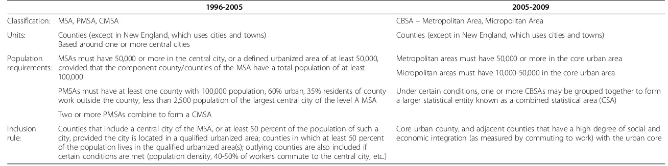
We update the earlier longitudinal analyses using CPS data through 2009, which was the latest year available at the time this research was done (the period covered by the ASEC files extended through 2008, versus 2009 for the MORG files). A substantial complication is introduced by changes in the geographic classification of areas in the CPS. Geographic in-formation in the CPS is reported by place of residence according to a classification system of“statistical areas”based on population density and commuting patterns. Before 2005, the system was based on four-digit Federal Information Processing Standard (FIPS) codes for the MSA, PMSA, or Consolidated Metropolitan Statistical Area (CMSA). In 2005, it chan-ged to one based on Core-Based Statistical Areas (CBSA), which have five-digit FIPS codes.

(9)

The pre-2005 MSA/PMSA/CMSA definitions grouped counties (or cities and towns in

New England) based around one or more “central cities” that can cross state lines.

Geographically-interconnected PMSAs are combined to form CMSAs, of which there are 18 in the United States. The post-2005 CBSA system is based on core urban areas instead of central cities. CBSAs are classified as either Metropolitan Areas or Micropolitan Areas, based on size requirements. Larger Metropolitan Areas are subdivided into Metropolitan Divisions, which are comparable to the subdivision of CMSAs into PMSAs in the pre-2005 definitions. One or more CBSAs may be grouped together to form a Consoli-dated Statistical Area (CSA). The definitions of these areas pre- and post-2005 are spelled out in Table 1.

The Census Bureau provides a crosswalk mapping post-2005 CBSAs to their pre-2005

MSA/PMSA counterparts.22The crosswalk contains 935 unique CBSAs (both

Micropoli-tan Areas and MetropoliMicropoli-tan Areas), but the 2005–2009 CPS data report only 275 unique

CBSAs, in large part because the CPS does not report Micropolitan Area CBSAs. Of the 275 unique CBSA FIPS codes, 245 CBSAs could be mapped directly to an MSA or CMSA using the crosswalk provided. Another 16 CBSAs were manually mapped using the New

England Cities and Towns Area (NECTA) definitions based on names.23The last step in

applying the crosswalk consists of consolidating PMSAs in the pre-2005 period into CMSAs, because the post-2005 CBSAs in the CPS data do not include Metropolitan Division distinctions. All PMSAs belonging to the 18 CMSAs in the United States were therefore rolled up into their appropriate CMSAs pre- and post-2005 in order to have consistent geographic areas across time.

These steps resulted in 215 unique MSA/CMSA areas. Geographic identifiers are

sup-pressed (for confidentiality reasons) for 35 of these – some before and some after the

change in geographic classification. Again, though, this is not pertinent to our analysis, be-cause this suppression occurs only for smaller cities that get dropped bebe-cause of too few observations. Thus, we have 180 MSAs or CMSAs defined on a consistent basis over the years we study.

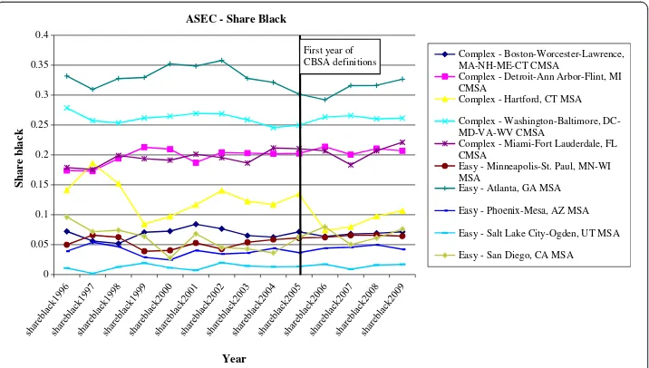
To assess the accuracy of geographical linkages over time, we chose five MSAs/CMSAs for which the conversion was complicated and five that were simple, and computed the shares black, Hispanic, and with low educational attainment (high school degree or equivalent), as well as weighted population estimates, over time in both the ASEC and MORG data. We wanted to check for breaks at the time of the switch in geographic classi-fication, which could point to inconsistent geographic definitions over time. There was no indication of unusual changes surrounding the switch in geographic definitions in 2005, for either the simple or the complicated CMSA aggregations. Figure 1 provides an ex-ample of one of these analyses, focusing on the share black in the ASEC data. This share is a useful metric, because residential segregation by race implies that incorrect changes in the geographic areas would likely deliver noticeable changes in the share of the population that is black. A more problematic issue, discussed below, is the accurate measurement of the living wage in these MSAs/CMSAs, in cases where living wages are in place in only some cities in the MSA/CMSA, or differ across them.

The empirical analysis is done with individual-level data. However, the analysis requires the estimation of percentiles of the wage or predicted wage distribution for MSAs/CMSAs, by month or year. To ensure a reasonable level of accuracy in doing this, we required that

an MSA/CMSA had at least 50 observations on individuals age 16–70 in all months of the

(10)

Table 1 Pre- and post-2005 geographic classification systems

1996-2005 2005-2009

Classification: MSA, PMSA, CMSA CBSA–Metropolitan Area, Micropolitan Area

Units: Counties (except in New England, which uses cities and towns) Based around one or more central cities

Counties (except in New England, which uses cities and towns)

Population requirements:

MSAs must have 50,000 or more in the central city, or a defined urbanized area of at least 50,000, provided that the component county/counties of the MSA have a total population of at least 100,000

Metropolitan areas must have 50,000 or more in the core urban area

Micropolitan areas must have 10,000-50,000 in the core urban area

PMSAs must have at least one county with 100,000 population, 60% urban, 35% residents of county work outside the county, less than 2,500 population of the largest central city of the level A MSA

Under certain conditions, one or more CBSAs may be grouped together to form a larger statistical entity known as a combined statistical area (CSA)

Two or more PMSAs combine to form a CMSA

Inclusion rule:

Counties that include a central city of the MSA, or at least 50 percent of the population of such a city, provided the city is located in a qualified urbanized area; counties in which at least 50 percent of the population lives in the qualified urbanized area(s); outlying counties are also included if certain conditions are met (population density, 40-50% of workers commute to the central city, etc.)

Core urban county, and adjacent counties that have a high degree of social and economic integration (as measured by commuting to work) with the urban core

Notes: For additional details, seehttp://www.census.gov/population/www/metroareas/mastand.htmlandhttp://www.census.gov/population/www/metroareas/metroarea.html(viewed on October 5, 2010).

Neumark

et

al.

IZA

Journal

of

Labor

Policy

2012,

1

:11

Page

10

of

34

http://ww

w.izajolp.com

/content/1

(11)

sample period 1996–2009. To have comparable analysis samples for the MORG and the ASEC data files, we required that this be met for both data files. This requirement was met by 39 of the unique MSAs/CMSAs after the geographic matching and roll-ups.

Data on living wages

Cities, rather than metropolitan areas, are the political units that adopt most living wage laws.We characterize the living wage laws prevailing in a metropolitan area based on the liv-ing wages passed by the major cities in the metropolitan area. Given the change in geo-graphic coding, it is not entirely straightforward to define a list of cities on which to focus for the entire analysis period. Prior to the change, the classification of larger cities was based on the definition of“central cities”(Frey et al., 2004), but with the switch to CBSAs larger cities were classified as“principal cities.”We needed to choose a set of cities within the 39 MSAs/CMSAs for which to code living wage laws in detail. We chose all central or princi-pal cities subject to two criteria: a population of at least 250,000 residents according to 2000 Decennial Census data;24and if no city in the metropolitan area had at least 250,000 resi-dents, the largest city in the metropolitan area. These criteria led to 52 cities within the 39 MSAs/CMSAs; both the cities and the MSAs/CMSAs are reported in Table 2.

For these cities,we needed historical information on living wage laws and other charac-teristics of the laws, such as whether they apply to recipients of financial assistance.25We first reviewed city websites for evidence of a living wage law and to identify a contact for follow-up. For cities where we initially found no evidence of a living wage law, we attempted to contact the City Clerk, City Manager, City Attorney, or Procurement/Public Works/Economic Development Officer by telephone to confirm whether the city had a living wage law at any time since 1995. If we were unable to reach the city representative by telephone, we followed up with email correspondence. At times, the first point of con-tact within a city directed us to another concon-tact, at which point we would repeat the process (call, followed by email). If the representative confirmed that the city never had a

0 0.05 0.1 0.15 0.2 0.25 0.3 0.35 0.4

Share black

Year ASEC - Share Black

Complex - Boston-Worcester-Lawrence, MA-NH-ME-CT CMSA

Complex - Detroit-Ann Arbor-Flint, MI CMSA

Complex - Hartford, CT MSA

Complex - Washington-Baltimore, DC-MD-VA-WV CMSA

Complex - Miami-Fort Lauderdale, FL CMSA

Easy - Minneapolis-St. Paul, MN-WI MSA

Easy - Atlanta, GA MSA

Easy - Phoenix-Mesa, AZ MSA

Easy - Salt Lake City-Ogden, UT MSA

Easy - San Diego, CA MSA First year of

CBSA definitions

Figure 1Assessment of Matching of Geographic Classifications, ASEC Data, Share Black.

(12)

Table 2 The 52 cities in the analysis sample, and their 39 MSAs/CMSAs

MSA/CMSA City MSA/CMSA City

Albuquerque, NM MSA Albuquerque Milwaukee-Racine, WI CMSA Milwaukee (1995)

Atlanta, GA MSA Atlanta Minneapolis-St. Paul, MN-WI MSA Minneapolis (1997)

Boise City, ID MSA Boise Minneapolis-St. Paul, MN-WI MSA St. Paul (2007)

Boston-Worcester-Lawrence, MA-NH-ME-CT CMSA Boston (1998) New York-Northern New Jersey-Long Island, NY-NJ-CT-PA CMSA Newark (2003)

Charlotte-Gastonia-Rock Hill, NC-SC MSA Charlotte New York-Northern New Jersey-Long Island, NY-NJ-CT-PA CMSA New York (2002)

Chicago-Gary-Kenosha, IL-IN-WI CMSA Chicago (1998) Oklahoma City, OK MSA Oklahoma City

Cincinnati-Hamilton, OH-KY-IN CMSA Cincinnati (2002) Omaha, NE-IA MSA Omaha

Cleveland-Akron, OH CMSA Cleveland (2000) Orlando, FL MSA Orlando (2003)

Columbus, OH MSA Columbus (2004) Philadelphia-Wilmington-Atlantic City, PA-NJ-DE-MD CMSA Philadelphia (2005)

Dallas-Fort Worth, TX CMSA Dallas Phoenix-Mesa, AZ MSA Phoenix

Dallas-Fort Worth, TX CMSA Fort Worth Phoenix-Mesa, AZ MSA Mesa

Dallas-Fort Worth, TX CMSA Arlington Pittsburgh, PA MSA Pittsburgh

Denver-Boulder-Greeley, CO CMSA Denver (2000) Portland-Salem, OR-WA CMSA Portland (1996)

Denver-Boulder-Greeley, CO CMSA Aurora Providence-Fall River-Warwick, RI-MA MSA Providence

Detroit-Ann Arbor-Flint, MI CMSA Detroit (1998) Raleigh-Durham-Chapel Hill, NC MSA Raleigh

Grand Rapids-Muskegon-Holland, MI MSA Grand Rapids Sacramento-Yolo, CA CMSA Sacramento (2004)

Honolulu, HI MSA Honolulu Salt Lake City-Ogden, UT MSA Salt Lake City

Houston-Galveston-Brazoria, TX CMSA Houston San Diego, CA MSA San Diego (2005)

Kansas City, MO-KS MSA Kansas City (2005) San Francisco-Oakland-San Jose, CA CMSA Oakland (1998)

Las Vegas, NV-AZ MSA Las Vegas San Francisco-Oakland-San Jose, CA CMSA San Francisco (2000)

Los Angeles-Riverside-Orange County, CA CMSA Los Angeles (1997) San Francisco-Oakland-San Jose, CA CMSA San Jose (1998)

Los Angeles-Riverside-Orange County, CA CMSA Santa Ana Seattle-Tacoma-Bremerton, WA CMSA Seattle

Neumark

et

al.

IZA

Journal

of

Labor

Policy

2012,

1

:11

Page

12

of

34

http://ww

w.izajolp.com

/content/1

(13)

Table 2 The 52 cities in the analysis sample, and their 39 MSAs/CMSAs(Continued)

Los Angeles-Riverside-Orange County, CA CMSA Anaheim St. Louis, MO-IL MSA St. Louis (2000)

Los Angeles-Riverside-Orange County, CA CMSA Long Beach Tampa-St. Petersburg-Clearwater, FL MSA Tampa

Los Angeles-Riverside-Orange County, CA CMSA Riverside Washington-Baltimore, DC-MD-VA-WV CMSA Baltimore (1995)

Miami-Fort Lauderdale, FL CMSA Miami (2006) Washington-Baltimore, DC-MD-VA-WV CMSA Washington (2006)

For cities that enacted a living wage, the year of enactment is shown in parentheses.

Neumark

et

al.

IZA

Journal

of

Labor

Policy

2012,

1

:11

Page

13

of

34

http://ww

w.izajolp.com

/content/1

(14)

living wage law, we “closed”the research on the city. If the representative indicated that there was, or had been, a living wage law, we added the city to the list for further research. For the cities with evidence of a living wage law, we obtained as much possible informa-tion from 1995 through 2010 from the city website or directly through a city representative. Using the city website, we reviewed the current living wage law found in the city’s municipal code or code of ordinances which, at times, contained a reference to the ordinance creating

the code.26The documents reviewed in the search typically generated information on the

living wage history (e.g., council agendas/minutes, budget presentations, or living wage or-dinance summaries), or reference forms containing the living wage rates (e.g., posters, memoranda, or living wage rate change bulletins), from which we gained additional detail. Once we established the broad picture, we used specific dates to track down the actual ordi-nances adopted and the living wage rates established during a given year. If necessary, we contacted city representatives by telephone or email to confirm findings or provide informa-tion that was not attainable from the city web pages.

Using this information, we coded the wage levels for the 26 cities that meet our criteria with living wages among the MSAs/PMSAs that we study, for each year and month from

January 1995 through December 2009.27We also coded whether or not the living wage law

applies to business assistance recipients.28The new information on living wage laws empha-sizes the potential value of updating the research on living wages. Of these 26 cities, 14 had enacted living wages prior to 2002, and 12 did so afterwards. Table 2 shows the year of en-actment of living wages for the cities in our analysis that enacted them. Thus, between the cities with new living wage laws, plus the additional observations on cities that passed them earlier and increased the level of the living wage subsequently, there is a good deal more

in-formation on the effects of living wages – and of course information that is more

contemporary.

Results: wage and employment effects

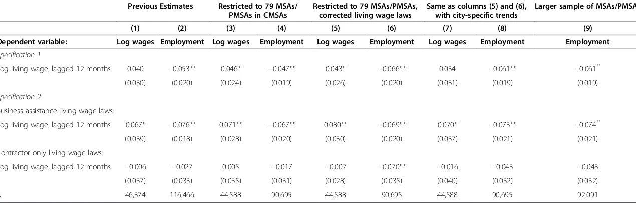
The first two columns of Table 3 repeat the basic estimates, from Adams and Neumark (2005a), of the effects of living wages on wages of workers in the bottom decile of the wage distribution, and the bottom decile of the skill (predicted wage) distribution; these estimates were discussed in Section II. The data cover all residents of MSAs and

PMSAs identified in the CPS ORG data in the 1996–2002 period, in city-month cells

with 25 or more observations. The key living wage variable in the model, for which estimates are reported in the table, is the log of the maximum of the living wage or the

minimum wage prevailing in the city, lagged 12 months.29The maximum of the two is

used to capture the effective wage floor, and the 12-month lag is used based on evi-dence that the effects of living wages do not occur instantly but emerge over about one

year.30 The regressions include controls for city, year, month, minimum wages, and

other individual-level controls. The specification also includes differential linear time trends for cities passing or not passing living wage laws, or passing different types of living wage laws. The first row reports the estimates from a single regression on the liv-ing wage variable, without distliv-inguishliv-ing the types of livliv-ing wage laws. In the second and third rows, instead, each column reports results from a specification that distin-guishes between contractor-only and business assistance living wage laws (by interact-ing the livinteract-ing wage variable with dummy variables for these types of laws, constructed to be mutually exclusive).

(15)

Table 3 Estimated effects of living wages on log wages and employment, lowest decile of wage distribution or predicted wage distribution (for employment), living wages defined at MSA/PMSA level, prior estimates and re-estimations for 1996-2002

Previous Estimates Restricted to 79 MSAs/ PMSAs in CMSAs

Restricted to 79 MSAs/PMSAs, corrected living wage laws

Same as columns (5) and (6), with city-specific trends

Larger sample of MSAs/PMSAs

(1) (2) (3) (4) (5) (6) (7) (8) (9)

Dependent variable: Log wages Employment Log wages Employment Log wages Employment Log wages Employment Employment

Specification 1

Log living wage, lagged 12 months 0.040 −0.053** 0.046* −0.047** 0.043* −0.066** 0.034 −0.061** −0.061**

(0.030) (0.020) (0.024) (0.019) (0.026) (0.020) (0.031) (0.019) (0.019)

Specification 2

Business assistance living wage laws:

Log living wage, lagged 12 months 0.067* −0.076** 0.071** −0.067** 0.080** −0.069** 0.070* −0.073** −0.074**

(0.039) (0.018) (0.028) (0.020) (0.030) (0.020) (0.037) (0.021) (0.021)

Contractor-only living wage laws:

Log living wage, lagged 12 months −0.006 −0.027 0.005 −0.017 −0.007 −0.070** −0.016 −0.043 −0.043

(0.037) (0.033) (0.035) (0.031) (0.028) (0.035) (0.040) (0.032) (0.032)

N 46,374 116,466 44,588 90,695 44,588 90,695 44,588 90,695 92,091

The estimates in columns (1) and (2) are from Adams and Neumark (2005a, Tables2and4). The data on labor market outcomes and other worker-related characteristics come from the Current Population Survey (CPS) monthly Outgoing Rotation Group files (ORGs/MORGs), from January 1996 through December 2002. Only observations on city-month or city-year cells with 25 or more observations are retained. The living wage variable is the maximum of the log of the living or minimum wage, and so equals the minimum wage when there is no living wage. The regressions include controls for city, year, month, log minimum wages, and other individual-level controls. All specifications also allow differential linear time trends for cities passing or not passing living wage laws, or passing different types of laws, except columns (7) and (8). The entries in the first row are from a specification with a single living wage variable, and the entries in the second and third rows are from a specification that interacts the living wage variable with dummy variables for the type of living wage. The MSAs/PMSAs beginning in columns (3)-(4) are the MSAs and PMSAs that constitute the 39 CMSAs that we can track for the entire sample period and that meet the data sufficiency requirement (50 valid wage observations per MSA/PMSA and month). The list of these 79 MSAs/PMSAs used in columns (3)-(6) is available from the authors upon request. There are 86 MSAs/PMSAs in column (9), where we do not impose the same data sufficiency requirement on the employment and wage samples. Estimates are weighted by individual sample weights.‘**

’(‘*

’) superscript indicates estimate is statistically significant at five-percent (ten-five-percent) level. Reported standard errors are robust to nonindependence (and heteroscedasticity) within city cells (clustered by city).

Neumark

et

al.

IZA

Journal

of

Labor

Policy

2012,

1

:11

Page

15

of

34

http://ww

w.izajolp.com

/content/1

(16)

The wage equation is a log-log specification, so the coefficients are elasticities. For example, the upper-left estimate means that a 100% increase in the living wage (e.g., from a $5 minimum wage to a $10 living wage) would increase wages in the bottom de-cile of the wage distribution by 0.04 log points, or approximately 4%. The coefficients from the employment regressions measure the change in the probability of employment in response to a one-unit increase in the log living wage (or a 100% increase).

For the first specification, the estimates in columns (1) and (2) indicate that living wages lead to higher wages and lower employment; only the estimated employment ef-fect is statistically significant. In the second specification, business assistance living wage laws have significant positive effects on wages, and significant negative effects on employment, whereas the effects of the narrower contractor-only laws are smaller and insignificant (and the wage effect is very close to zero). The magnitudes imply that a 100% business assistance living wage increase boosts wages in the bottom decile of the distribution by 6.7%, and reduces employment in the bottom decile by 7.6 percentage points.

The remainder of Table 3 shows the consequences of some changes to the sample necessitated by the aggregation of MSAs/PMSAs to MSAs/CMSAs, and of other changes to the data or specification. First, columns (3) and (4) report estimates using the exact same data and specifications, but restricting attention to the MSAs/PMSAs that are aggre-gated to MSAs/CMSAs in what follows. This entails very small reductions in the sample size, as only 12 very small MSAs/PMSAs that were included in the original analysis are dropped. For the wage analysis, 79 MSAs/PMSAs meet this criterion and other sample size restrictions. More MSAs/PMSAs meet the sample size restrictions for the analysis of employment, because the samples for these outcomes are larger. However, we report most results for the consistent set of MSAs/PMSAs. We also report key results for the largest possible samples of MSAs/PMSAs within these MSAs/CMSAs, on the argument that these give us the most reliable estimates for each outcome. The changes in the estimates shown in columns (3) and (4) are inconsequential.

Columns (5) and (6) incorporate some slight changes in the living wage data based on the new research on the history of living wage laws. Most of the estimates are essentially unchanged, with the exception of the employment effect for contractor-only living wage laws, which is now the same magnitude as for business assistance laws and statistically sig-nificant. Columns (7) and (8) report specifications in which less-restrictive linear trends– now, simply city-specific linear trends – are substituted for the differential linear time trends for cities passing or not passing living wage laws, or passing different types of laws. For business assistance living wage laws, which are our main focus, this change has little bearing on the estimates. Again, though, the results for contractor-only laws are more sen-sitive (and, consequently, so are the results for living wages overall). In particular, there is now no evidence of a statistically significant positive wage effect for living wages overall, or of significant (positive) wage effects or (negative) employment effects for contractor-only laws. As reported in column (9), the employment effects are robust to including an additional seven MSAs/PMSAs that meet the data sufficiency criterion for employment but not wages. The conclusion from these estimates is still that business assistance living wage laws lead to positive wage effects and negative employment effects, both of which are statistically significant. The estimates with city-specific trends become our “baseline” estimates for purposes of comparison going forward.31

(17)

Table 4 explores the consequences of extending the data through 2009, which requires the aggregation to MSAs/CMSAs. Now the key variable in the model, for which estimates are reported in the table, is the log of the maximum of the minimum wage or the weighted living wage (weighted by population share of the MSAs or PMSAs in the MSA/CMSA), lagged 12 months as before. This weighted living wage variable is calculated by multiplying the living wage in an MSA/PMSA by the population share of that MSA/PMSA in the total MSA/CMSA population living in MSAs or PMSAs (based on 2000 Census data), and sum-ming the weighted living wages across all MSA/PMSAs in the MSA/CMSA.

As columns (3) and (4) show, once we aggregate and extend the data, the evidence changes relative to the baseline estimates (columns (1) and (2)). For wages, the estimated effects of the overall living wage and the two separate living wage variables are all positive but statistically insignificant, and the estimate for business assistance living wage laws – which was larger and statistically significant in the previous analyses–declines. For the em-ployment effects, although all of the estimates are negative, none is large compared to the overall and business assistance living wage effects estimated earlier, and the estimate for business assistance living wages, which should have the highest coverage, is not significant.

To explore the consequences of the aggregation of MSAs and PMSAs to MSAs/CMSAs necessitated by the changes in the CPS data, in columns (5) and (6) we keep everything the same as in columns (1) and (2)–in particular, using the data only through 2002–and the

onlychange we make is to do this aggregation. The estimates also change substantially rela-tive to columns (1) and (2) and are not very different from those when we extend the data through 2009. This illustrates that it is the aggregation that changes the estimates, rather than extension of the sample period.

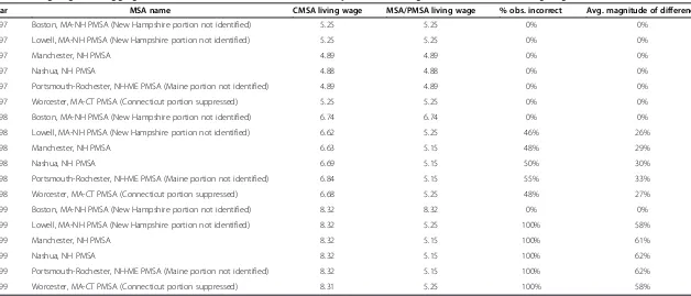
The aggregation to MSAs/CMSAs turns out to pose a severe empirical problem for a very simple reason: it is difficult to measure living wages at the MSA/CMSA level be-cause of many instances in which MSAs or PMSAs within an MSA/CMSA adopt living wages at different times (and also at different levels, although the differences in timing

are the more serious issue). Table 5 illustrates the problem, for the case of Boston.32

Boston passed a living wage in 1998, while the other MSAs and PMSAs in the CMSA did not. For the years in the sample period through 2002 (when the original analysis ended), somewhat under half the observations in the CMSA are outside of the Boston PMSA. In the original analysis through 2002, the Boston living wage was assigned only to the Boston PMSA. However, with the change in geographic classification, the other five MSAs/PMSAs were aggregated with the Boston PMSA, resulting in the living wage being assigned to all six of them beginning in July 1998, when the Boston living wage was implemented. Table 5 shows that in 1997 (and the same is true earlier) when there was no living wage in Boston, there is no measurement problem. The living wage takes effect midway through 1998, so the percentage of observations with the wrong living wage (and the average magnitude of the error) is fairly small in that year. In 1999 (and subsequently), the error rate and magnitude of the error becomes considerably larger.

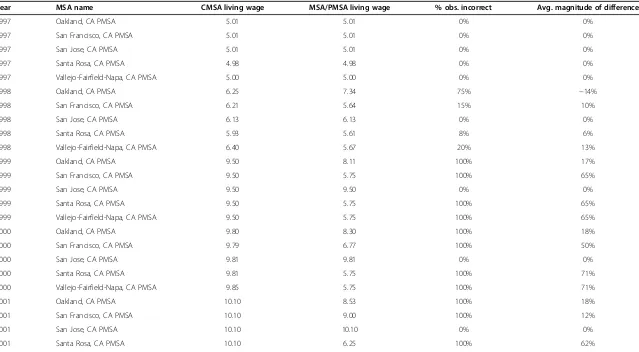
Table 6 shows a similar problem for the aggregated San Francisco-Oakland-San Jose CMSA. In this case, the adoption of living wages differs, with each of the three major constituent MSAs/PMSAs adopting living wage laws at different times. Nonetheless, the same severe measurement problem emerges. One difference in this case, though, is that the error decreases over time, as the major MSAs/PMSAs each adopt a living wage.

(18)

Table 4 Updated estimates of effects of living wages on log wages and employment, lowest decile of wage distribution or predicted wage distribution (for employment)

“Baseline”estimates, Table3, columns (7) and (8), 1996-2002

Living wage variables aggregated to CMSA level, 1996-2009

Living wage variables aggregated to CMSA level, 1996-2002

Living wages defined at MSA/ PMSA level, 1996-2004

(1) (2) (3) (4) (5) (6) (7) (8)

Dependent variable: Log wages Employment Log wages Employment Log wages Employment Log wages Employment

Specification 1

Log living wage, lagged 12 months 0.034 −0.061** 0.026 −0.019** 0.009 −0.039* 0.037 −0.052**

(0.031) (0.019) (0.019) (0.009) (0.036) (0.021) (0.034) (0.017)

Specification 2

Log living wage, lagged 12 months 0.070* −0.073** 0.021 −0.005 0.025 −0.026 0.051 −0.055**

(0.037) (0.021) (0.023) (0.012) (0.042) (0.026) (0.041) (0.023)

Log living wage, lagged 12 months −0.016 −0.043 0.022 −0.029** −0.052 −0.053 0.020 −0.048**

(0.040) (0.032) (0.027) (0.014) (0.057) (0.035) (0.056) (0.023)

N 44,588 90,695 86,614 188,769 44,588 90,695 53,038 109,725

Note: See notes to Table3.‘*’(‘**’) superscript indicates estimate is statistically significant at five-percent (ten-percent) level. All specifications have city-specific trends. Reported standard errors are robust to nonindependence (and heteroscedasticity) within city cells (clustered by city).

Neumark

et

al.

IZA

Journal

of

Labor

Policy

2012,

1

:11

Page

18

of

34

http://ww

w.izajolp.com

/content/1

(19)

Table 5 Living wages and aggregation errors, boston CMSA and MSAs/PMSAs, years surrounding enactment of Boston living wage

Year MSA name CMSA living wage MSA/PMSA living wage % obs. incorrect Avg. magnitude of difference

1997 Boston, MA-NH PMSA (New Hampshire portion not identified) 5.25 5.25 0% 0%

1997 Lowell, MA-NH PMSA (New Hampshire portion not identified) 5.25 5.25 0% 0%

1997 Manchester, NH PMSA 4.89 4.89 0% 0%

1997 Nashua, NH PMSA 4.88 4.88 0% 0%

1997 Portsmouth-Rochester, NH-ME PMSA (Maine portion not identified) 4.89 4.89 0% 0%

1997 Worcester, MA-CT PMSA (Connecticut portion suppressed) 5.25 5.25 0% 0%

1998 Nashua, NH PMSA 6.69 5.15 50% 30%

1999 Nashua, NH PMSA 8.32 5.15 100% 62%

Boston’s living wage was adopted in 1998. The living wage variables are averaged over months in a year. The MSA/PMSA living wage sometimes shows small deviations before there is a living wage because the table reports the average minimum wage (or living wage, if there is one), the state minimum wage can change mid-year, and the sample proportions in different months can vary across areas.

Neumark

et

al.

IZA

Journal

of

Labor

Policy

2012,

1

:11

Page

19

of

34

http://ww

w.izajolp.com

/content/1

(20)

Table 6 Living wages and aggregation errors, San Francisco-Oakland-San Jose CMSA and PMSAs, years surrounding enactment of living wages in PMSAs

Year MSA name CMSA living wage MSA/PMSA living wage % obs. incorrect Avg. magnitude of difference

1997 Oakland, CA PMSA 5.01 5.01 0% 0%

1997 San Francisco, CA PMSA 5.01 5.01 0% 0%

1997 San Jose, CA PMSA 5.01 5.01 0% 0%

1997 Santa Rosa, CA PMSA 4.98 4.98 0% 0%

1997 Vallejo-Fairfield-Napa, CA PMSA 5.00 5.00 0% 0%

1998 Oakland, CA PMSA 6.25 7.34 75% −14%

1998 San Jose, CA PMSA 6.13 6.13 0% 0%

1999 Oakland, CA PMSA 9.50 8.11 100% 17%

1999 San Jose, CA PMSA 9.50 9.50 0% 0%

2000 Oakland, CA PMSA 9.80 8.30 100% 18%

2000 San Jose, CA PMSA 9.81 9.81 0% 0%

2001 Oakland, CA PMSA 10.10 8.53 100% 18%

2001 San Jose, CA PMSA 10.10 10.10 0% 0%

Neumark

et

al.

IZA

Journal

of

Labor

Policy

2012,

1

:11

Page

20

of

34

http://ww

w.izajolp.com

/content/1

(21)

Table 6 Living wages and aggregation errors, San Francisco-Oakland-San Jose CMSA and PMSAs, years surrounding enactment of living wages in PMSAs

(Continued)

2002 Oakland, CA PMSA 10.10 8.69 100% 16%

2002 San Jose, CA PMSA 10.10 10.10 0% 0%

The Oakland and San Jose living wages were adopted in 1998, and San Francisco’s in 2000. The living wage variables are averaged over months in a year. The MSA/PMSA living wage sometimes shows small deviations before there is a living wage because the table reports the average minimum wage (or living wage, if there is one), the state minimum wage can change mid-year, and the sample proportions in different months can vary across areas.

Neumark

et

al.

IZA

Journal

of

Labor

Policy

2012,

1

:11

Page

21

of

34

http://ww

w.izajolp.com

/content/1

(22)

There is a similar aggregation problem for other cities for which MSAs/CMSAs in-clude MSAs/PMSAs with different living wages. There are only 20 MSAs/CMSAs that

do not suffer from either problem, and only five of these have living wage laws; hence

we could not reliably estimate living wage effects using this subset of observations. As a consequence of this aggregation problem, the best alternative is likely to revert to the specification at the MSA/PMSA level, and to use as long a sample period as pos-sible prior to the change in geographic coding. For the analysis of wages and employ-ment, this implies extending the sample period through 2004, which unfortunately

does not provide as much “updating” as we would like. Nonetheless, this does give us

information on an additional four cities that passed living wage laws in 2003 or 2004 (Columbus, OH, Newark, NJ, Orlando, FL, and Sacramento, CA). Results are reported in the final two columns of Table 4. There are some changes relative to the baseline estimates in columns (1)-(2). For the living wage variable overall, and the business as-sistance living wage variable, the estimated wage effects are smaller, and the wage effect for business assistance living wage laws is no longer statistically significant, although the estimated coefficient still implies a sizable effect: a 100% living wage increase boosts wages in the bottom decile of the wage distribution by 5.1%. For employment effects, in contrast, the evidence is somewhat stronger. There is still evidence of a statistically significant negative effect of business assistance living wage laws on employment of less-skilled individuals and of living wage laws overall. But now the estimate is similar (al-beit a bit smaller), and statistically significant, for contractor-only living wages as well.33

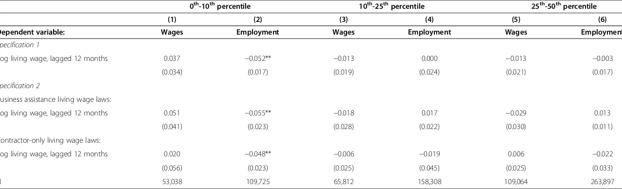
We also estimated these specifications for different ranges of the wage and skill distribu-tion. This is of interest for two reasons. First, as confirmation that we are truly detecting effects of living wages on low-wage, low-skilled workers in the results reported above, we should clearlynotfind evidence of positive wage andnegativeemployment effects higher up in the wage or skill distribution. Second, a living wage can generate demand shifts toward higher-skilled workers, increasing their wages and employment (e.g., Fairris and Bujanda, 2008). And as Adams and Neumark (2005a) showed, many poor families have workers who earn relatively low wages or have relatively low skills but are not necessarily in the bottom 10thof the distribution.34Thus, policies that end up helping workers who are in a higher part of the wage distribution can reduce poverty.35

As reported in Table 7, we found little evidence of effects higher up in the wage or skill dis-tribution. The wage effects were small and centered on zero, and not statistically significant. The estimated employment effects were also small and statistically insignificant, although more uniformly negative. These results suggest that effects of living wages on the distribution of family incomes stem mainly from the effects of living wages on the lowest-wage and lowest-skilled workers. Moreover, the absence of any evidence higher up in the wage or skill distribution paralleling that for the lowest-wage, lowest-skill workers makes it less likely that our results for the latter groups reflect spurious effects of changes in economic conditions correlated with living wages. That is, these results serve as a placebo test.

Based on our updated evidence, there is now stronger evidence of disemployment effects, and it is not only limited to business assistance living wage laws. And there is weaker evidence of wage effects. Two points related to these findings merit discussion. First, in the earlier work, the stronger evidence of effects of business assistance living wage laws was attributed to the likely higher coverage of these laws as well as other fea-tures of those laws, although the evidence was not decisive (see Adams and Neumark,

(23)

Table 7 Estimated effects of living wages on log wages and employment in other ranges of the wage or predicted wage distribution (for employment) living wages defined at MSA/PMSA level, updated, 1996-2004

0th_-10th_percentile ₁₀th_-25th_percentile ₂₅th_-50th_percentile

(1) (2) (3) (4) (5) (6)

Dependent variable: Wages Employment Wages Employment Wages Employment

Specification 1

Log living wage, lagged 12 months 0.037 −0.052** −0.013 0.000 −0.013 −0.003

(0.034) (0.017) (0.019) (0.024) (0.021) (0.017)

Specification 2

Log living wage, lagged 12 months 0.051 ₋0.055** ₋0.018 0.017 ₋0.029 0.013

(0.041) (0.023) (0.028) (0.022) (0.030) (0.011)

Log living wage, lagged 12 months 0.020 ₋0.048** ₋0.006 ₋0.019 0.006 ₋0.022

(0.056) (0.023) (0.025) (0.045) (0.025) (0.033)

N 53,038 109,725 65,812 158,308 109,064 263,897

See notes to Table3.‘**’(‘*’) superscript indicates estimate is statistically significant at five-percent (ten-percent) level. All specifications have city-specific trends. Columns (1)-(2) include observations less than or equal to the 10th

percentile; columns (3)-(4) from greater than the 10th

to less than or equal to the 25th

; and columns (5)-(6) from greater than the 25th

to less than or equal to the 50th

. Note that the sample sizes do not change in close proportions to the percentage of observations in each range based solely on the percentiles. This occurs because the percentiles are calculated for fairly small samples in many instances (since they are computed for city-month cells), so there are often large numbers of ties in the rankings of observations. We define the samples in the different columns as explained earlier in the note, so in some cases the share of observations in a range can substantially exceed or fall short of the strict definition. (For example, if there are many observations on either side of the 10th

percentile, but the 25th

percentile is higher, then more than one-tenth of the observations will be in the lower decile.) Reported standard errors are robust to nonindependence (and heteroscedasticity) within city cells (clustered by city).

Neumark

et

al.

IZA

Journal

of

Labor

Policy

2012,

1

:11

Page

23

of

34

http://ww

w.izajolp.com

/content/1

(24)

2005a). There is no indication one way or another that coverage of contractor-only laws has increased because of some inherent broadening of the laws. However, the laws may now have stronger effects, because in the earlier years of living wage laws, there may have been a greater preponderance of non-renewed contracts that were not covered. It is true that the business assistance provisions also often applied only to new assistance. But as discussed earlier, these business assistance provisions may have broader effects.

Second, the early wave of research on living wages was based on relatively few periods cov-ering a fairly small number of cities. As a result, the results were described as somewhat provisional, requiring more data and more analysis for confirmation.36Consequently, it is not surprising that there are some changes in the answers relative to the earlier research, al-though in general most of the qualitative results persist, including the results for poverty dis-cussed below. At the same time, the above discussion regarding the problems of aggregating geographic data on U.S. cities, using CPS data, indicates that we have been unable to add a large number of years of data with reliable measurement of living wages.

Results: Effects on low-income families

We next report estimates of the effects of living wages on family income (poverty) and on government benefits to families. These estimates tell us how the various and possibly com-plicated wage and employment (and hours) effects on individuals ultimately affect families. Table 8 focuses on whether living wages reduce the probability that families are poor. These models are estimated for the full sample, not the lower decile of the wage or skill distribution (or other ranges). Column (1) repeats the estimates from Adams and Neumark (2005a). The estimates are negative for living wages generally and for business assistance living wages (although the point estimate is larger for contractor-only living wages). To in-terpret the estimates, the−0.024 estimate for business assistance living wage laws, for ex-ample, implies that a 100% increase in this type of living wage reduces the poverty rate by 2.4 percentage points. Columns (2) and (3) report the results for the restricted sample (79 cities), and then with city-specific trends. These results are consistent with business assist-ance living wage laws being the only types of living wage laws that reduce poverty.

We next return to the issue of aggregation of urban areas into MSAs/CMSAs, which is necessary to update the results fully. Doing the aggregation without changing the sample period (column (4)) leads to estimated effects–in the direction of reducing poverty–that are a bit larger. In columns (5)-(6), we show the aggregated estimates through 2009, and

then the disaggregated estimates (which we think are most reliable) through 2003,37 the

last year for which the disaggregated data are available. The basic qualitative conclusion –

that business assistance living wage laws reduce urban poverty – is robust across all of

these estimates. However, the estimates through 2003, without aggregating, no longer show a statistically significant effect of business assistance living wage laws in reducing poverty. Nonetheless, we do not want to dismiss the aggregated results, which show a sta-tistically significant effect of business assistance living wages in reducing poverty.38 More-over, in both columns (5) and (6) we no longer–relative to the earlier estimates reported in column (1)–find any effect of contractor-only living wage laws on poverty.

Finally, we examined information on income-support and other assistance programs. Given that many income-support programs require low family income to qualify, or tie benefits to income, we might expect the beneficial effects of living wages to be more