Manuscript Title & Authors

e-ISSN: 2278-7461, p-ISSN: 2319-6491

Volume 7, Issue 1 [January 2018] PP: 78-85

A kriging asa surrogate modeling tool

Varun

1

(Transportation Engineering, Dept. of Civil Engineering, IIT Delhi, India)

Corresponding Author: Varun1

ABSTRACT: -

KEYWORDS: Blind-kriging,co-kriging, limit kriging, surrogate model.

--- ---Date of Submission 25-01-2018 ---Date of acceptance: 19-02-2018 --- ---

I.

INTRODUCTION

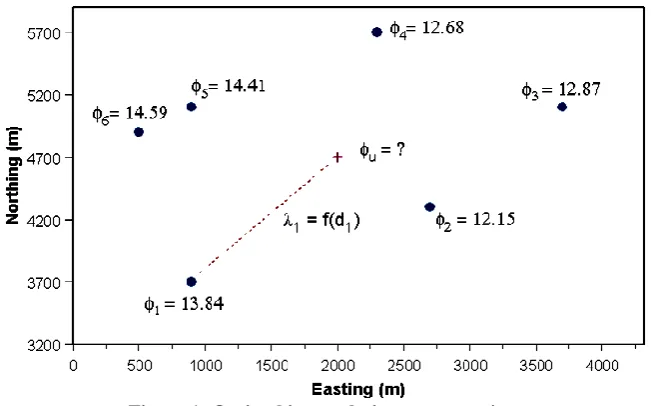
Kriging is the method of optimal interpolation to get the estimation of a variable at an unmeasured location from the Z-value observed at various surrounding data points, weighing to the special covariance values, to estimate partly at u with x &y coordinates at 2000m, 4700m as in figure-1, using interpolation on regression at nearest 6 points inzone data. All interpolation method gives the results as a weighted sum of data values from surrounding locations or functions that gives decreasing trend whereas a kriging assigns weight according to data driven function, good estimate at results are obtained if the data is distributed dense through study area(1).

Figure 1: Optimal interpolation on regression

a) Characteristics of kriging(11)  Accepts irregularly spaced data

 Considers only surrounding values which are supposed to be used for estimation.  Calculates an error of estimate

 Autocorrelation between known data values for estimation of unmeasured values

b) Kriging advantages

 Kriging treats clusters as like as the point‟s help to carry estimate the effects of data clustering.  It gives, known value of estimation errors (kriging variance) along with the z variable

 Gives estimation of errors for stochastic simulation of possible realizations of Z(u)(2). c) Applications(11)

 Hydrogeology – interpolation for an aquifer altitudes

 Environmental monitoring – use of modern statistical interpolation methods for distributions of radioactive contamination and disease incidence rates etc.

 Soil science with agriculture field – investigation of soil quality.

 Ecology – to predict missing values where explanatory variables are used.

Kriging was developed by Krige, mining engineer in South Africa, in field of geostatistics and extension of kriging are still in review. On searching for word „Kriging‟ via Google on March 10, 2015 gave 527000 hits, which shows the popularity of this mathematical method.The basics of kriging till recent extensions is reviewed in this paper and these basics and extension may convince analysts in deterministic or random simulation of the potential usefulness of Kriging(3).Kriging is a mathematical model for determining the noise free data and is known as Gaussian processes, learning for machine community have no differences in terms as associated methodology is adopted except the technology. Kriging is popular model but it is not publicallyavailable. Its interpolations are easy to use but many are outdated and often limited to one specific type with most well known as surrogate model.This paper address the need for presenting the implementation of object-oriented kriging and its various extensions with easily extendable framework (4).

In general, kriging models are usedas surrogatemodel for a response and its statistics asthe nonlinearity of its variance is higher than response. The interpolation with krigingis more reliable which provides an accurate prediction for nonlinear functions. In addition,kriging is superior to other approximation methods for the design problem and for the kriging model statistics,sample points are determined based on simulations of kriging model of response that not onlyreduce the tedious computing time but also facilitates robust optimization.All functions in the design formulation are expressed in mathematical forms, and when kriging models are run for statisticsthey result to a simple optimization problem (5).

Kriging models provide an easy and productive way for approximation of deterministic and computation intensive simulation code.Kriging use data such as gradient data, hessian data, multi-field data etc. and hence as an advantage of additional information provide accurate results in more accurate manner, when first-order and second-order derivative data is used in kriging. The improvement in the result of model due to gradient data may not be worth the cost of computation and the fittings (6). Presently, kriging model have been adopted in electromagnetic devices for its functional optimization. These models basically provide functional relationship for robust optimization for predicting the design variables by using the objective function based on sample points and save time consumed in direct calculation(7).

Most of the engineering design problems review experiments for evaluation, several regression and simulation to arrive at an outcome loaded to heavy costs, hence, such surrogate model need to evaluate the design objectives to save time and money for results as closely as possible and to bring cost cheaper than any other models. Surrogate models are prepared by bottomup datadriven approach considering in the mind that only input and output behaviors is important with working of simulation code and is even assumed to be not known. Hence, sometimesthis bottomup approach isknown by behavior approach model or black-box approach modeling when only single driven variable is involved in modeling and that processes is known as the curve-fitting.

II.

LITERATURE REVIEW

a) Basics of kriging

Kriging surrogate model gives efficient deterministic simulation codes for computations and additional interpolation gives more advantages for kriging surrogate model which enhance the accuracy in the multifunction data and also improve the accuracy in kriging surrogate model with first order and second order derivative data. Kriging surrogate model is a statistics-based interpolationmethod (8).The kriging efficiency largely depends upon the actual capture load behavior to its correlation function. In this interested in investigation strength of kriging to develop the more accurate surrogate model with deterministic simulation code. There are the various type of simulation extension including simple kriging,ordinary kriging, universal kriging, regression kriging , co-kriging and blind kriging used by couckuyt(3).Ordinary kriging focus on simple type of kriging that is –

𝜔 𝑑 = 𝜇 + 𝛿 𝑑 (1)

b) Limit kriging(10)

A kriging model gives an interpolating predictor that can be used to afunction based on number of evaluations and can be stated as follows –

Y (x) = μ + Z(x) (2)

The function evaluate at „n‟ number of points {X1, ……….., Xn } and assume thatY= (Y1 ……….…..Yn)

be the values of corresponding function then kriging predictor at X for the function is as follows –

𝑦 𝑥 = 𝜇 + 𝑟 𝑥 −1𝑅−1(𝑦 − 𝜇1) (3)

Where, 1 is a column of first „n‟ number length and „R’is amatrix of „n x n’ with R(xi -xj), that the change in „μ‟

of simple than kriging predictor depending on the value of „x’, there after might be ableto improve the prediction. Therefore, consider a modified predictor formas follows –

𝑦 𝑥 = 𝜇 + 𝑟 𝑥 −1_𝑅−1_{(𝑦 − 𝜇(𝑥)1) (4)}

If 0 < r(x)1R-1 1 <2, and k →∞, taking limits on both sides of equation- 4, than predictor becomes as –

lim_𝑘→∞𝑦 𝑘 𝑥 = 𝜇 𝑥 + 1

𝑟 𝑥 ′𝑅−11𝑟 𝑥

′_𝑅−1 _{𝑦 − 𝜇 𝑥 1 (5)}

lim𝑘→∞𝑦 𝑘 𝑥 =𝑟 𝑥

′_𝑅−1_𝑦

𝑟 𝑥 ′𝑅−1₁ (6)

Anew simple predictoris obtained in equation – 6, with varying „μ‟ named as the limit kriging predictor.

c) Kriging surrogate model

In the kriging model, response function of a deterministic computer experiment is as –

Z(x) = b(x)T β+ ε(x) (7)

Where, the drift function is b(x)T β and ε(x) showing an average behavior of response „Z(x)‟ with random error „E[ε(x)] = 0‟and x is n number of dimension position vector and the basis function is b(x) = [b1(x), b2(x), . ……….. . , bK(x)]T . β = [β1, β2, ….. . . ,βK]

T

is unknown vector of regression coefficients.When the order of the polynomial is zero, one and two, among all types of kriging models, polynomial drift function is most popular. It becomes ordinary Kriging, first-order universal kriging and second-order universal krigingrespectively, the parameters of the universal kriging satisfy the following equations –

𝜆𝑖𝑏𝑚(𝐱𝑖 ) = 𝑏𝑚(𝐱) 𝑁

𝑖=1 (8)

𝜆𝑖𝐶𝑜𝑣 [𝑍 𝑋𝑖 , 𝑁

𝑖=1 𝑍(𝑋𝑗)] + 𝐾𝑚 =1𝛿𝑚𝑏𝑚 𝑋𝑖 = Cov[𝑍(𝐱), 𝑍(𝐱𝑗 )] (9)

m = 1, ………. , K, and j = 1, …………, N

Where, the order of the polynomial for drift function is K and number of sampling points is N,unknown Kriging weight coefficient is λ, Lagrange multiplier is δ,the basis function is b(xj ) and zero is mean value of stochastic component and xi and xj is covariance between two sampling points‟ as follows –

Cov[Z(xi ), Z(xj)] = ζ 2

R[R(xi , xj)] (10)

Where, the variance of Z(x) is ζ2, covariance function is R(xi , x j)(8) and sampling values of linear combination are –

𝑍∗ _{= 𝜆} 𝑖𝑍 𝑥𝑖 𝑁

𝑖=1 (11)

Once sampling point‟s kriging surrogate model is constructed, time-consuming numerical method will replace the performance analysis in most of engineering problems and order of polynomial for the drift function and correlation function strongly affect the accuracy of Kriging surrogate models (9).

d) Kriging with linear expression

The difference between loworderpolynomials with modern simulation for kriging, gives simple simulation output and multi-polynomial simulation output expressionin model is –

„ω‟ is output under laying simulation , s(…) is mathematical function by capture code to simulation, dj with (j = 1, 2, ……….. k) simulation input variable. D = (dij) simulation design matrix experiment with i = 1, 2, …………..n(2)

.

e) Gradient enhanced kriging

In the estimation of gradient enhanced kriging, ŷ (x*) at a point x* refers a simulation constraint function û, which gives a model –

𝑦 𝑥∗ _{= 𝜇 + 𝜓}𝑇_Ψ−1 _{𝑦 − 1𝜇}

(13)

Where, the relation between sample data and prediction is𝜓 at point x* and function value of sample data is y, correlation matrix is Ψ(5).The ordinary kriging model does not imply flat response surface but regression model refers universal kriging and in the deterministic simulation is quit useful for surrogate modeling, in the stationary covariance process for 𝛿 𝑑 .if θ> 0 , than there are several stationary covariance process for single input as –

 ρ(h) = max (1- θh,0):Linear correlation function

 ρ(h) = exp (- θh) :Exponential correlationfunction

 ρ(h) = exp (- θh2

) :Exponential correlationfunction

A most popular kriging function is –

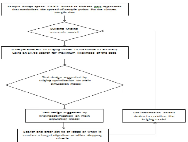
Figure 2: Flow chart showing process of Kriging

𝜌 ℎ = 𝑒𝑥𝑝 − 𝜃𝑗ℎ𝑗

𝑝𝑗 𝑘

𝑗 =1 = 𝑒𝑥𝑝 −𝜃𝑗ℎ𝑗

𝑝𝑗 𝑘

𝑗 =1 (14)

Where, 𝜃𝑗 is importance of input j and pj is reflect the smoothness of correlation function (2).

f) Surrogate modelling –

 Optimization with single-objective

Algorithm approach can be directly used on main simulation model instead of searching kriging model, in addition of this similar test was taken was starting with same initial sample population and EA was used to search the optimum design values with or without surrogate model. The initial sample size of 5, 10, 20 and 50 were taken in single objective optimization with surrogate model and algorithm was run with optimum design values, the same algorithm was run without surrogate model with same sample size and initial populationhaving like as like modelwith total number of optimization for stability of average performance of algorithmand the performance of both method is compared based on the total number of simulation required on main model to find optimum level of design.The performance of optimizations withthe single-objective, 10 runs of each set is shown as below –

Table 1:Results with and without a Kriging surrogate model(P*<0.05; P**<0.01).

Population size for initial sample

Main model samples, average number to find optimum,

mean and standard deviation t-test for two samples, P (T<=t),for two-tail

Without kriging model With kriging model

5 1154 (±887) 84 (±38) 0.0013**

10 1325(±1612) 68 (±36) 0.024*

20 584 (±348) 88 (±59) 0.0003**

50 625 (±409) 100 (±45) 0.0008**

The comparison ofbest performing Kriging optimization at population size of 20 is significant at the 99.9% confidence level.

 Optimization with Multi-objective

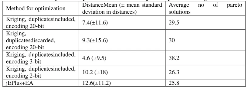
Multi objective optimization is used over objective where single-objective optimization can be reformulated with expected improvement for more than one objective. The EI basics giving the probability of objective for better design suggestion by EA current pareto frontusually combining with two or more objectives into a single objective is problematic as relative importance is needed to define for each objective with multi-objective EI.However, with a multi-objective EI, keepthe single-objective algorithm without pre-assigning weightings to each objective and then combinewith two objectives to enable same EA to use without surrogate model, which can be compared with the surrogate optimization method against a well-established multi-objective EA (10). The performance of the different types of multi-objective optimization are summarized in Table 2 considering the sampling budget is limited to 200 samples of the main simulation model. Algorithms that used a Kriging surrogate model are shaded in grey.

Table 2: Comparison of performance of multi-objective optimization algorithms.

Method for optimization DistanceMean (± mean standard deviation in distances)

Average no of pareto solutions

Kriging, duplicatesincluded,

encoding 20-bit 7.4(±11.6) 29.5

Kriging,

duplicatesdiscarded, encoding 20-bit

9.3(±15.6) 30

Kriging, duplicatesincluded,

encoding 3-bit 4.6 (±9.5) 38.2

Kriging, duplicatesincluded,

encoding 2-bit 10.2 (±18) 26.3

jEPlus+EA 12.6(±11.2) 25.8

g) Design for Kriging

The regression metamodel with first-order polynomial is as given in equation below –

𝑦𝑟𝑒𝑔 = 𝛽0+ 𝛽1𝑑1+ . . . 𝛽𝑘𝑑𝑘+ 𝑒𝑟𝑒𝑔 , (15)

Where, Y is the regression predictor, 𝛽.= (𝛽0, 𝛽1, … … . , 𝛽𝑘) is the vector and𝑒𝑟𝑒𝑔 , is the error. In the above equation , left side of equation equates the generation of input/output simulation data for fitting a kriging model, left side of equation only assumed that an adequate metamodel is more complicated than low order polynomial, however, it does not assume any specific metamodel or simulation model. Left side of equation focuses on design space formed by k-dimensional defined by„k‟ standardized simulation inputs if, 0≤ di.j ≤ 1 with i = 1,. . . n and j = 1, . . . k,this property implies that the design depends on the specific underlying process. Nevertheless, sequential procedures may be less efficient with computations and there are several approaches for sequential design of simulation experiments with important to distinguish between two different goals of simulation experiments, particular sensitivity analysis and optimization (2).

EXAMPLE

Compare the accuracy for kriging surrogate model andfor analytical test function given –

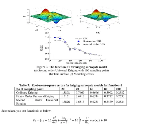
𝐹1= 3 1 − 𝑥1 2𝑒𝑥𝑝 −𝑥12− 𝑥2+ 1 2 − 10 𝑥1

5−𝑥₁3−𝑥₂5 𝑒𝑥𝑝 −𝑥1

2_{− 𝑥}

22 − exp⁡[− 𝑥1+ 1 2− 𝑥22]/3 Where, −3 ≤ X1 andX2 ≤ 3

Table 3: Root-mean-square errors for kriging surrogate models for function-1

No of sampling point 20 40 60 80 100

Ordinary Kriging 1.5898 0.7469 0.6696 0.3902 0.2582 First – Order UniversalKriging 1.5151 0.6713 0.6334 0.3712 0.2533 Second – Order Universal

Kriging 1.3826 0.6513 0.6231 0.3479 0.2524

Second analytic test functionis as below –

𝐹2= [𝑥2− 5.1 𝑥12 4π2+

5𝑥2 π− 6]

2_{+ 10 1 −} 1

8π cos 𝑥1 + 10 Figure 3. The function F1 for kriging surrogate model (a) Second order Universal Kriging with 100 sampling points

Where, −5 ≤ X1 ≤ 10 and 0 ≤ X2 ≤ 15

Table–4:Root-mean-square error errors for kriging surrogate models for F2

No of sampling point 20 40 60 80 100

OK 4.3869 0.4206 0.0981 0.0205 0.0257

First – Order Universal Kriging 4.5734 0.4218 0.0969 0.0192 0.0247 Second – Order Universal Kriging 4.9322 0.3212 0.0845 0.0205 0.0243 Root-mean-square error (RMSE) is a modeling error that is defined to access accuracies of model as follows –

𝑅𝑀𝑆𝐸 = [𝑧

∗ _𝑥

𝑖 − 𝑧 𝑥𝑖 ]2 𝑁𝑇𝑆

𝑖=1

𝑁𝑇𝑆

Where, Kriging surrogate model predicted value is Z∗ _(x

i) and Z (xi), NTS is number of uniform testing points and is a set of 40 × 40. Figure 3 and Table 3 compares the modeling errors for analytic function F1. Figure 4 and Table 4 shows the results of Kriging surrogate models clearly stating that kriging surrogate models decrease fast if number of sample points increases hence with increase in no. of samples, the error is very limited and approached to zero..

III. CONCLUSION

The paper provides discussions for the efficient use of kriging surrogate model showing that kriging surrogate model are better and accurate than any other theoretical or numerical methods. The conclusions concluded from the extraction of the paper are.as follows –

 The kriging surrogate model is to be applied to provide the relationship between model frequency and crack parameter to avoid the expensive Finite Element (FE) analysis.

 The multi-objective robust optimization technique can be applied to kriging surrogate model to reduce the computation time involved in calculation of the value of objective function.

 Example presents that the higher accuracy in second order universal kriging is obtained as compared to first order universal kriging model if number of sample points are increased.

 Kriging model can also be applied to practical random simulation models, which are more compacted than academic queuing and inventory models.

 Time consumed in kriging surrogate models is less than any other simulations.

 In the design problem with multi-objective, if the number of calls simulation is limited to 200 than use of a surrogate model allowsbetter approximation for Pareto front.

REFERENCES

[1]. Geoff Bohling, (2005). “KRIGING” , < http://people.ku.edu/~gbohling/cpe940>

[2]. Jack P.C. Kleijnen,(2009), “Kriging metamodeling in simulation: A review”European Journal of Operational Research 707–716, volume – 192 , page 707 - 716

[3]. Ivo Couckuyt, Tom Dhaene and Piet Demeester, (2014), “ooDACE Toolbox: A Flexible Object-Oriented Kriging Implementation” Journal of Machine Learning Research, volume - 15 : 3183-3186

[4]. Kwon-Hee Lee1, Gyung-Jin Park2 and Won-Sik Joo, (2005), “A Global Robust Optimization Using the Kriging Based Approximation Model” 6th World Congresses of Structural and Multidisciplinary Optimization Rio de Janeiro, Brazil

[5]. A. Tolk, S. Y. Diallo, I. O. Ryzhov, L. Yilmaz, S. Buckley, and J. A. Miller,(2014), “on the use of gradients in kriging surrogate models” Proceedings of the 2014 Winter Simulation Conference,IEEE, volume – 978: 2692 – 2701

[6]. Bin Xia, Ziyan Ren, Chang-Seop Koh, (2014) “Utilizing Kriging Surrogate Models for Multi-Objective Robust Optimization of Electromagnetic Devices” IEEE Magnetics Society, Volume-50, Issue-2Rasmus Bro, (2005) “surrogate model”, < http://www.models.kvl.dk/ercim/>

[7]. J. D. Martin and T. W. Simpson, (2005)“Use of Kriging models to approximate [8]. Deterministic computer models,” AIAA J., vol. 43, no. 4, pp. 853–863.

[9]. Es Tresidder1, Yi Zhang1, and Alexander I. J. Forrester2,(2012), “acceleration of building design optimisation through the use of kriging surrogate models” First Building Simulation and Optimization Conference, Loughborough, UK

[10]. V. Roshan Joseph, (2012) “Limit kriging” Technometrics, Taylor & Francis ,Volume 48, Issue 4, Page: 458-466

[11]. Ulrike Weise, (2001) “Kriging – a statistical interpolation method and its applications”< http://ibis.geog.ubc.ca/courses/geog570/talks_2001/kriging.html >