147203-7979-IJECS-IJENS © June 2014 IJENS
Comparative analysis of Scheduling Algorithms in
Network On Chip using Network Calculus
NeilaMoussa
1, Jamila Bhar
2, Farah Nasri
3, RachedTourki
4Abstract– The design of on chip interconnection architecture (NoC) should carefully take on consideration both hardware and communication constraints in order to build up a system that meets quality of service requirements. In the NoC architecture, the on chip switch available hardware and software resources drive up the global performances of the communication processes. Therefore it is crucial, before the physical design process, to carry out the required capacities such as buffer depth and management-tasks of a flit. In fact, one of the most critical parameters that can affect communication characteristics are the available memory space in addition to flit-time processing according to a given scheduling approach.
This paper deals with these concepts. It presents a study of mesh NoC using Network Calculus (NC) theory. We aggregate the individual temporal properties of each component given in switch model to obtain the formula of backlog size and the delay bound. Second we apply theses formulas to calculate the maximum end-to-end delay for NoC 2 ×2 communication scenarios and the buffer requirement on such switch. This helps to specify the best physical and logical characteristics that can achieve enhanced performances.
Index Term-- Network on Chip (NOC) and Network Calculus
I. Introduction
The immense capacity of integration offered by the semiconductors technology makes it possible from now to conceive integrated systems on chip (SoC). The realization of these systems is subjected to several performance constraints such as cost, production time and marketing. Therefore the interconnection between electronic components is a major concern of research. Thus, Networks on Chips (NoCs) have been introduced as an efficient solution for the growing problems of current interconnects in VLSI chips [1] [2]. In fact NoC is becoming a field of research which still requires a lot of intervention. The difficulty of the NoC design lies in compromise between optimal quality of service (QoS), high use of band-width and flexibility, while optimizing metric design (limitation of the consumption of energy, minimization of plugs’ size and silicon surface). Majority of current works are focused on switches in the networks on chip [3] [4] [5] [6] and [7], considering it is the key element in architectures. Switches occupy almost 90 percent of the space allotted to the network on chip. So NoC switches should be small, energy efficient, and fast. The complexity of the switch design mainly depends on the size of the buffer and the processing time of a flit. The evaluation of these proposed solutions and the NoC architecture, most researches uses directly simulation [7] [9] [10] or hardware implementation [3]. However, other researchers treat the analytical prediction. Authors in [27]
compared four analytical methods (Queuing Theory (QT), Network Calculus (NC), Schedulability Analysis (SA), Data Flow Analysis (DF)) for the noc evaluation and conclude that any one of them can’t replace all other and they believe that comprehensive frameworks that combine two or more formalisms would be most desirable. In [25] and [26] authors analyzed with network calculus the NoC performance for respectively self extractor flow and variable bit rate flow. However they don’t focus on the scheduling policy in the switch. As such, our paper is a challenge to bridge two domains: on-chip networks worlds and mathematic theory. We present in this paper the evaluation of mesh NoC architecture with an analytical approach. To this end, we use network calculus theory where the detailed can be found in [11], [12] and [13]. With the use of both ( s; ρ) arrival curve and the specification and modeling of the scheduling policy in the queue, we hope to instigate the necessary memory size and the limitation of the transfer times in the NOC. So according to the desired performances, this estimate helps to take the good choice at the moment of design similar to defining the best technique for a limited time design. This paper is organized as follows: In section II we formulate the flow model and switch architecture. Then we show in section III the analytical performance of the proposed NoC architecture. In section IV we illustrate the modeling scenarios of the application, and the performance results. Finally we conclude this work and highlight some future objectives.
II. NETWORK CALCULUS BACKGROUND
Le Boudec and Thiran [11] have developed the network calculus theory and based it on min-plus algebra. Network calculus is a mathematical framework to derive worst-case bounds on maximum latency, backlog in a single node or a network of nodes. It can be classified into two types: deterministic network calculus and statistical network calculus. The basic elements in this former are arrival curves as an abstraction of application traffic and service curves as an abstraction of network elements. Here, we give the necessary introductory material used in this article.
II.1. Definition1 (Min-Plus Convolution and deconvolution)
The functions f(t) and g(t) are wide-sense increasing defined for real number t ≥ 0, and f (0) = g(0) = 0. then their convolution under min-plus algebra is defined as:
147203-7979-IJECS-IJENS © June 2014 IJENS and their de-convolution is defined as:
( f
⊘
g)(t) = sup s≥0{ f (t +s)−g(s)} (2)II.2. Definition 2 (Arrival curve)
Let α is a wide-sense increasing function defined for t≥ 0, we say that a flow R is constrained by arrival curve α if and only if for all t ≥ s,
(R(t)−R(s)) ≤α(t −s) (3)
II.3. Definition 3 (service curve)
A well-defined service curve is latency rate β R,T
βR,T (t) = R(t −T)+(4)
Where R is the service rate and T the maximum response delay.
II.4. Theorem 1 (Delay bound)
Assume a traffic flow constrained by arrival curve α(t), traverses a system that provides a service curve β (t). at any time t, the delay D(t) satisfies,
D(t)t≥0 ≤ infτ≥0 {α(t) ≤β (t +τ} (5)
The delay bound define the maximum delay that would be experienced by a flit arriving at time t. Graphically the delay bound is the maximum horizontal deviation between α(t) and β (t).
II.5. Theorem 2 (Backlog bound)
Assume a traffic flow constrained by arrival curve α(t), traverses a system that provides a service curve β (t). The backlog B(t) for all t satisfies,
B(t) ≤ sup t≥0 {α(t)−β (t)} (6)
The backlog bound is the amount of bits that are held inside the node. the required buffer size of a switcher is determined by the maximum backlog. Graphically, the backlog bound is the maximum vertical deviation between α(t) and β (t).
II.6. Theorem 3(Output bound)
Assume a traffic flow constrained by arrival curve α(t), that traverses a system that provides service curve β (t). The output flow is constrained by the following arrival curve,
α*(t) = sup
s≥0 {α(t +s)−β (s)} (7)
II.7. 1.7. Definition 7 (Concatenation)
Assume a traffic flow traversing tow systems witch offers respectively a service curve β1(t) and β2(t). The concatenation of the tow systems offers the β(t) flows service, defined by,
β (t) = (β1
⊗
β2)(t) = inf0≤s≤t {β1(t −s)+β2(s)} (8)III. MODELING
III.1 Flow modeling: Arrival Curve
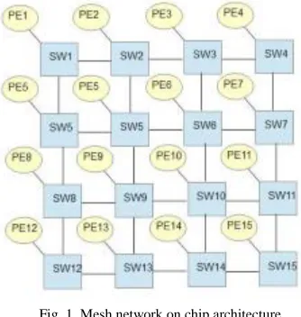
Typically NoC architecture consists of multiple processing elements (PEs) also called IPs, which communicate through switch. Communication in NoC is based on to tow kinds: traffics flows between PE and switch and also traffics between two or more switchers. Some works exploited the analytical modeling of systems on chip to analyze the performances. In [24] a traffic configuration schemes for evaluating networks on chips was proposed and demonstrated. Analytic approach is the most efficient but limited in capability of calculation [23]. So it, seems to be possible to consider these traffics as to be stair arrival curve function, that could be extended by an affine curve function. The mean idea has be found their origin in the bucket bored concept [11]. The interest of this alternate will appear practically in a calculations’ simplification and the delays’ expressions.
Fig. 1. Mesh network on chip architecture
This mechanism of regulation of the arrival data is used before in the case of SoC in [17] [16] [22]. Then from previous descriptions, we know that both routers and IP nodes have the ability to transmit the flows. Assuming the maximum quantity of data flow arrived that can be sent by each switcher or node at one moment T; t = 0; is supposed to be formed by the following arrival curve: α(t) =σ +ρt where ρ is the average data rate, and σ describes the maximum burst size of the data flow. In the case of real time communication, the parameters σ and ρ of the affine function will be given from the specificities of the application.
III.2. Switcher model
147203-7979-IJECS-IJENS © June 2014 IJENS header flit sets up the routing paths at each switcher. First, flits
are classified into various service classes with crossbar and then assigned to a queue that is specifically dedicated to that service class. Then, flits will cross multiplexer with scheduling policy.
The switch architecture and switch model proposed on fig3 integrates five elementary components. First the input of incoming flits, the demultiplexer was classified
Fig. 2. The model of NoC switch architecture
flit in service classes, class based FIFO storage, the multiplexer that ensures of output scheduling and finally the multiplexer processing routing. To identify the switch service curve, we should model it for each component. The resulting service curve is a concatenation of them in an additional operation.
IV. SERVICE CURVE IDENTIFICATION
IV.1. FIFO service curve
For the waiting in queue FIFO, the associated curve of service could be defined by the following expression:
( ) ( ) {
The equation shows the absence of treatment before a time equivalent to one horloge cycle. Each input buffer has one classifier. The classifier is modeled as demultiplexer that take one delay to execute head (H) flit, data (D) flit or end of packet (EOP) flit. The associated service curve is defined by:
( ) ( ) {
The equation shows that the flit management in the demultiplexing block is raised one .
IV.2 Multiplexer service curve
To provide quality of service (QoS) guarantees in a communication network, a fundamental need is to provide service differentiation as well as fairness among traffic classes. A basic technique that enables the share of a common resource among multiple traffic classes is a scheduling discipline. To date, a lot of scheduling disciplines have been proposed in the research literature, among which, the Strict Priority (SP) and Weighted Round Robin (WRR) are perhaps
the tow most widely adopted disciplines. Each flow upper-constrained with where is the number of priority/class and a weight is given to each flow. The number of classes of service may be different from the number of priority levels. For each class based FIFO, a maximum of flits is defined as the allowed flit number that can be managed during a scheduling cycle. In the following, the flit size noted L is constant. Moreover, the multiplexer stability is conditioned by Cout=C, this means that the available bandwidth should be bigger than the input data rate. Otherwise, the backlog will be increasing infinitely and thus the delay bound may become infinite. Two scheduling policies are supported: the strict priority (SP)
For this policy, none guarantee is offered to on flow. The selection order will simply depend on the priority (weight) order. Also, we have to distinguish the service curve offered to each flow. The strict priority policy guarantees to the flow flits with the highest priority. In Strict-Priority algorithm, the selection order is based on the priority of weight order. The algorithm services the highest priority queue until it is empty, after which, it moves to the next highest priority queue. The WRR policy is based on Round robin technique flow will be served in a cyclic way. The multiplexer treats in success each port in a pre-established order constrained by the weights of such queue. This can ovoid the starvation caused in the SP policy.
Theflit management in the multiplexer can be divided on three steps. In fact, in addition to the effective output transmission, two initial stages are required: Flit’s presence detection at the input and flit reading. The associated times to theses operations are given by tin= t=t. We note i the index of the class service considered ( i∈ N). Now, we analyze in particular the delays for each flow according to whether the policy of the node is SP or WRR.
a- WRR scheduler service curve
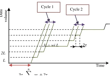
It is possible to identify the service offered by the multiplexer starting from the guarantees delivered by the policy of scheduling namely the quantum of cells treated in each cycle. Thus the multiplexer offers a service to a flow i characterized by cycle. The multiplexer offering a service to a flow i is characterized by an average transmission rate
∑ . The parameter integrates the flit
147203-7979-IJECS-IJENS © June 2014 IJENS Fig. 3. The WRR multiplexer service curve
At the end, the service curve of this component may be expressed in the equation (4). The notations used on the equation (4) are expressed as follow:
TABLE I.
UTILISATION NOTATIONS
Notations SIGNIFICATIONS
K1
Completely treated Flits number during the last Round Robin cycle.
K2
Completely past Round Robin cycle number.
M
Maximum data quantity of flow i treated during one Round Robin cycle: wi L
Q Maximum duration of treatment of flow other than flow i during a cycle:
∑
P
R
Processing time of one flit:
Rate of output:
Proposition 1 WRR scheduler service curve
The weighted round robin scheduler service curve offered tothe class i by a multiplexer of weight wi is given by:
( ) ∈ * ( ) }
With , ( ∑ )
∑
Precedent equation expresses two types of latency in the service curve. Each one expresses a part of the total spend time. The period expresses the always paid latency corresponding to the electronic latency. The parameter Q ( ∑ ), include the pessimistic supposition that the flit has just missed the turn of his flow. Concurrently to theses more traditional latency appears in the second time, a scheduling looping latency.
This latency is caused by the others flows treatment and the preceding flow’s flits already treated. For D flit and EOP flit spend one delay for searching the associated H flit before the scheduling treatment so the service curve for D flits and EOP flits can be expressed as follow:
Proposition 2 WRR scheduler service curve
The weighted round robin scheduler service curve offered to the ith class by a multiplexer of weight wi is given by:
( ) ∈ * ( ) }
With , ( ∑ )
∑
b- SP scheduler service curve
The switcher in figure 2 present four service class height, medium, normal and low priority, so we have four service curve for each flow. The multiplexer offering a service to a flow i is characterized by an average transmission rate . Like round robin policy integrates the flit management. Thus, the service offered by the component considered for a data flow i for low, normal, medium and height priority can be characterized by the curve of service shown in Fig.4.a ,Fig.4.b, Fig.4.c and Fig.4.d
Fig. 4.aThe service curve for low priority flux Fig. 4.b The service curve for normal priority flux 3L= wi L
L 2L
Time
∑
Cycle 1
D
at
a
v
o
lu
me
Cycle 2
L 2L
Time Service curve of
normal priority flux service curve of
D
at
a
v
o
lu
me
∑
D
at
a
v
o
lu
me
L 2L
147203-7979-IJECS-IJENS © June 2014 IJENS
Fig. 4.c Theservice curve for medium priority flux Fig. 4.d The service curve for height priority flux
The notations used on the equation (4) are expressed as follow:
TABLE II.
UTILISATION NOTATIONS
Notations SIGNIFICATIONS
K1
Completely treated Flits number during the last SP cycle.
K2 Completely past SP cycle number
L1max Maximum data quantity of flow i of height priority transmitted
L2max Maximum data quantity of flow i of medium priority transmitted
L3 max
Maximum data quantity of flow i of normal priority transmitted
L4 max Maximum data quantity of flow i of low priority transmitted
Proposition 3 SP scheduler service curves
The Strict priority scheduler presents four service curves. Each class service has individual service curve.
The multiplexer of height priority is given by:
( ) ∈ * ( ) } With ,
The multiplexer of medium priority is given by: ( ) ∈ * ( ) } With ,
The multiplexer of normal priority is given by:
( ) ∈ * ( ) } With , ( )
The multiplexer of low priority is given by:
( ) ∈ * ( ) }
With ,
( )
IV.4 Demultiplexer service curve
For the execution time in the de-multiplexer, the associated service curve is defined by:
( ) ( ) {
The equation shows that the H flit, D flit or EOP flit management in the demultiplexing block is raised by a time
IV.5 Switch service curve
The switch model proposed on fig3 integrates five elementary components: a file modeling the store and forward a demultiplexer for classifying flows, a class based FIFO, a multiplexer for the arbitration and a demultiplexer for the routing. Let us note that in this proposal, the routing is already integrated and it acts in the multiplexer service curve. If we notes the file service curve the classifier service curve, the median FIFO service curve and the multiplexerservice curve, the service curves theorem composition impliesthat switcher service curve(shown in fig 3) for H flits is given by , that is to say:
= inf 0≤s≤t {β1 (t −s)+β2 (t −s)+ β3 (t
−s)+ β4 (t −s)+ β5 (s )}
Proposition 4Switch service curve
In the case of Weighted round robin policy, the service curve provided by a switch to a flow i joining to a weight wi
is given by:
( ) ∈ * ( ) + L
2L
Time Service curve of
medium priority flux service curve of
D
at
a
v
o
lu
me
L 2L
Time
Service curve of height priority
flux service curve of
D
at
a
v
o
lu
147203-7979-IJECS-IJENS © June 2014 IJENS With , ( ∑ )
∑
In the case of strict priority policy, four switch service curve given by:
For height priority ( ) ∈ * ( ) } with ,
For medium priority ( ) ∈ * ( ) } with ,
For normal priority ( ) ∈ * ( ) } with , ( )
For low priority ( ) ∈ * ( ) } with
( )
V. BACKLOG AND DELAY BOUND
In order to make easier their computing, periodic model of service curve are typically approximated[17] [14].In this work we have avoided to base the description of the service curve on the establishment of some approximations ,hopping to build up rigorous delay and backlog estimation.
V.1Baclog bound
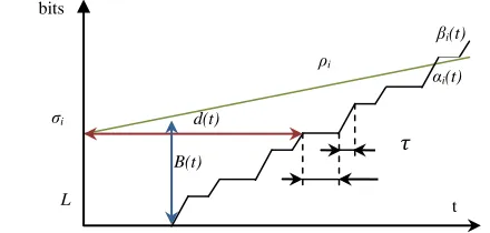
The condition used carry on corresponds to the minimization of the buffer memory size to hold for each input port. This information depends on the maximum size of the back of treatment combined to the flit retransmission of a flow i. As being defined in [11] and illustrated on Fig6, the back of treatment corresponds to the vertical distance between the arrival curve and the service curve.
Proposition 4 Switch backlog
For WRR policy, the Backlog bound for an i flow of wi weight, constrained by an arrival curve α(t) = ρt +σ and Switch traversing is given by:
( ∑
)
For SP policy, the backlog bound for an I flow, constrained by an arrival curve α(t) = ρt +σ and Switch traversing is given by:
For height priority ( )
For medium priority ( )
For normal priority (( ) )
For low priority
(( ) )
However it is to note that proposition 2 does not give the minimal total size of the buffer to avoid any saturation.
Indeed, it simply offers the maximum quantity of data on standby for a flow i, and not for all entering flows.
V.2 Delay bound
The delay bound for a data flow with an arrival curve α (t) that receives the service curve is the maximum horizontal distance between βi(t) and α(t) like seen in fig.5 The expression was already rappelled in section II.
D(t)t≥0 ≤ inf τ≥0 {α(t) ≤β (t +τ} (5)
Fig. 5. Curve of arrival and service, distances horizontal and vertical.
Proposition 5Switch delay bound
For WRR, the crossing delay bound of a flow i of weight wi, constrained by an arrival curve ( ) ( ) at the Switch crossing moment is raised by:
( ) ∑
(⌊
⌋ ) (⌊ ⌋ )
For SP policy, we have four crossing delay bound of a flow i, constrained by an arrival curve ( ) ( ) at the switch crossing moment is raised by:
For height priority: ( ) (⌊ ⌋ )
For medium priority: ( ) (⌊ ⌋ )
For normal priority: ( ) ( ) (⌊ ⌋ )
For low priority: ( ) ( ) (⌊ ⌋ )
5- NUMERICAL EXAMPLES
In this section, we consider a simple application mapped on NoC and show how to estimate delay and buffer by using surveyed mathematical formalisms. Figure 9 shows the task graph and also communication. As illustrated in fig9, the cores 0, 2,5 and 8 are selected to be traffic sources. Cores 3,4,5,6 and 7 considered as sinks. We can see, in this traffic pattern, that core 0 and 2 are selected as a multi traffic source and core 4 is selected two times to be a traffic sink.
t L
bits
βi(t)
αi(t)
ρi
σi d(t)
147203-7979-IJECS-IJENS © June 2014 IJENS
(a) (b)
Fig. 9. a) Task graph of an application mapped on an (b) NoC platform.
The basic traffic supported by this architecture consists of messages divided in flits presenting all the same size: 32 bits, 16bits, 64 bits. Links and routers are organized in a 3 × 3 mesh structure. Table III shows attributes of the traffic flows, including flow priority, source and destination of the flow, the values of sigma and rho, as well as route of the flow in the network. Data flows are represented by sequences of hops
from a source core to a destination core. These data flows are computed using a deterministic routing protocol to direct flits between switches.
The exchanges considered are described in table (Tab III). The scale values of sigma and rho are adopted from the work presented in [17] and describing on chip communication with network calculus concepts.
Table III
Flow Weight Priority Source Destination Sigma(flits) Data (flits)
Rho(flit/cycle) Route
f1 w4 High 0 4 40 100 0.16 R0,R1,R4
f2 w3 medium 2 1 48 100 0.24 R2,R1
f3 w1 Low 2 5 40 700 0.24 R2,R5
f4 w4 High 5 3 40 100 0.16 R5,R4,R3
f5 w2 Normal 0 7 48 200 0.24 R0,R1,R4,R7
f6 w1 low 0 6 48 500 0.24 R0,R3,R6
f7 w3 medium 8 4 40 100 0.16 R4,R7,R8
As described in section 2, each switch classed buffer will be constrained by the weight wn where N is the class based
weight. Classes based buffer weights value are 1, 2, 3, 4 related respectively to the w1, w2, w3r w4.
The output buffer of this data has will be obtained like seen in [11].
α*(t)= σ+Dρ
with D correspond to a total delay for the total input curves
Taking into account the topology and the policy of routing XY, it is possible to represent the traffics ways.
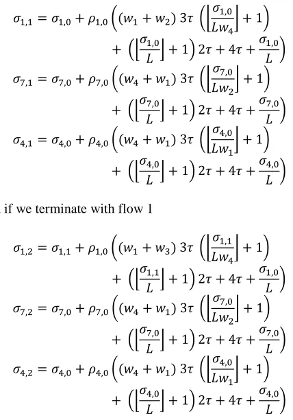
For example, on the switch (1) we have three flow f1, f7 and f2, they have respectively the priority height, normal and law We give in the next same equation of σ:
7
0
6
5
4
3
8
2
1
3 4 5
0 1 2
6 7 8
IP0
IP6
IP3 IP5
IP8 IP4
IP7
IP2 IP1
f1 f2
f3
f4
f5
f6
147203-7979-IJECS-IJENS © June 2014 IJENS (( ) (⌊
⌋ ) (⌊ ⌋ ) ) (( ) (⌊
⌋ ) (⌊ ⌋ ) )
(( ) (⌊ ⌋ )
(⌊ ⌋ ) )
And if we terminate with flow 1
(( ) (⌊ ⌋ )
(⌊ ⌋ ) ) (( ) (⌊
⌋ ) (⌊ ⌋ ) )
(( ) (⌊ ⌋ ) (⌊ ⌋ ) )
With these value and the other value of we can determine the value of the worst end to end delay and buffer size of each switch for three scheduling technique (RR, WRR, SP).
Fig. 10. Buffer size of each switch.
We can see in the fig 10 that the buffer size of all switches will be less when we use the WRR and same the SP scheduling technique.
The buffer size change from one switch to another, this can be explained by the charge of each switch or explicitly the number of flow that traverse.
Fig. 11. Worst delay of each flow.
Figure 11 show a major difference between the three scheduling technique. Highest worst case was obtained with WRR and the lowest was obtained with round robin scheduler. So we can deduce that the use of WRR or also SP scheduler will be limited for the real time flow that doesn’t allow highest delay.
6 CONCLUSION AND FUTURE WORKS
The main contribution of this paper is the presentation of an analytic approach for formal performance prediction applied for on-chip network design. We have used the network calculus theory in order to shape the NoC switch behavior and to predict its performances. Further, we had showed how this theory can be used to optimize the required buffer size according to the flow characteristics. This helps to correlate the required resources in order to meet the performances of the applications. As a future work we are looking to the hardware design of this switch in order to check the physical characteristics.
Future work is the use of this analyze method more realistic value dependant on a real time NOC application. Also we can extend the use of the network calculus theory on the power evaluation on SoC and providing more support for design space exploration.
REFERENCES
[1] [1] L. Benini and G.DeMicheli ”Networks on Chips: A New SoCParadigm”, IEEE Computers, pp. 70-78, Jan. 2002
[2] Z. Lu ”Design and Analysis of On-Chip Communication for Network-on-Chip”Platforms Stockholm 2007
[3] P. Vellanki, N. Banerjee and K.S. Chatha, ”Quality-of-Service and ErrorControl Techniques for Network-on-Chip Architectures”,ACM 2004
[4] J. Hu and R. Marculescu , ”Application-Specific Buffer Space allocationfor Networks-on-Chip Router Design,” in the Proc. Of ICCAD, pp. 354 -361, 2004.
[5] L-F. Leung and C-Y. Tsui ”Optimal Link Scheduling on Improving Best-Effort and Guaranteed Services Performance in Network-on-Chip Systems”GLSVLSI’04, April 26-28, 2004, ACM.
[6] E.Bolton, I.Cidon, R.Ginosar and A. Kolodny ”QNoC: QoS architectureand design process for network on chip” Journal of system architectureACM,50, 105 - 128, February 2004.
0.00 20.00 40.00 60.00 80.00 100.00 120.00 140.00
WRR SP Round
robin
Switch9
Switch8
Switch 7
Switch 6
Switch 5
Switch 4
0 5 10 15 20 25 30 35 40
1 2 3 4 5 6 7 8
flux
WRR
SP
147203-7979-IJECS-IJENS © June 2014 IJENS [7] E. Rijpkema, K. Goossens, A. Radulescu, ”Trade offs in the design
of arouter with both guaranteed and best-effort services for networks on chip”,Design, Automation and Test in Europe (DATE’03), March 2003, pp. 350-355.
[8] A. Kumar and R. Mahapatra ”An Integrated Scheduling and Buffer ManagementScheme for Input Queued Switches with Finite Buffer Space”,Computer Communications 29 (2005) 42-51.
[9] B. Ahmad, A.T. Erdogan, S. Khawam ”Architecture of a DynamicallyReconfigurable NoC for Adaptive Reconfigurable MPSoC” Conference onAdaptive Hardware and Systems (AHS’06),IEEE 2006.
[10] T. Tao Ye, L. Benini , G. De Micheli, ”Packetization and routing analysisof on-chip multiprocessor networks”. Journal of Systems Architecture 50(2004) 81-104.
[11] J-Y. Le Boudec and P. Thiran T. J Network Calculus; A Theory of Deterministic Queuing Systems for the Internet”, LNCS 2050, 2001.
[12] Cruz, R. ”A calculus for network delay, part I : network elements inisolation”. IEEE Transactions on Information Theory, 37(1), 114-141.1991a
[13] Cruz, R. ”A calculus for network delay, part II : Network analysis. IEEETransactions on Information Theory, 37(1), 132-141.1991b [14] J.P. Georges, T. Divoux, E. Rondeau, ”Confronting the
performancesof a switched Ethernet network with industrial constraints by using theNetwork Calculus. IJCS, International Journal of Communication Systems,John Wiley & Sons,
[15] S. Chakraborty, S. Kunzli, L. Thiele, ”A. Herkersdorf, and P. Sagmeister.Performance evaluation of network processor architectures: Combining,simulation with analytical estimation”. Computer Networks, 41(5), 2003.
[16] M. Gries, C. Kulkarni, C. Sauer, and K. Keutzer. ”Comparing analytical modeling with simulation for network processors: A case study”. In Proc.ofthe Designer’s Forum at DATE, 2003. [17] T. Henriksson, P. van der Wolf, A. Jantsch, and A. Bruce
”Networkcalculus applied to verification of memory access performance in SoCs”. InProceedings of the 5th IEEE Workshop on Embedded Systems for Real-Time Multimedia, October 2007. [18] A. Maxiaguine, S. Chakraborty and L. Thiele ”DVS for Buffer-
Constrained Architectures with Predictable QoS-Energy Tradeoffs” 2005ACM
[19] S. Murali and G. De Micheli, ”Bandwidth-constrained mapping of coresonto NoC architectures,” in Proc. DATE, pp. 16-20, Feb. 2004.
[20] M. Coenen, S. Murali, A. R.adulescu and K. Goossens G. De Micheli ” Abuffersizing Algorithm for Networks on Chip using TDMA and creditbasedendtoend Flow Control” , Seoul, Korea. ISSS’06, ACM.2006,
[21] G. Varatkar, R. Marculescu ”Traffic Analysis for On-chip Networks Designof Multimedia Applications” New Orleans, Louisiana, USA DAC ACM2002
[22] A. Maxiaguine, S. Kunzli and L. Thiele ”Rate Analysis for Streaming Applicationswith On-chip Buffer Constraints” Asia and South Pacific DesignAutomation Conference (ASP-DAC), Yokohama, Japan, January 2004
[23] W. J. and Towels, B ”Principles and Practices of Interconnection Networks”.Morgan Kaufman Publishers, 2004.
[24] Z. Lu and A. Jantsch. ”Traffic configuration for evaluating networks onchips”. In Proceedings of the 5th International Workshop on System onChip (IWSOC’05), Banff, Canada, July 2005.
[25] B.Akesson ,K. Goossens and M. Ringhofer ”Predator: A PredictableSDRAM Memory Controller” ISSS’07ACM 2007 [26] Po-Tsang Huang and Wei Hwang ”Predator: ”2-Level FIFO
ArchitectureDesign for Switch Fabrics in Network-on-Chip”, International Symposiumon Circuits and Systems (ISCAS), 2006. [27] A. Andriahantenaina, H. Charlery, A. Greiner, L. Mortiez et al.
”SPIN:a Scalable, Packet Switched, On-Chip Micro-network , Design Automationand Test in Europe Conference (DATE’2003), march 2003, Munchen, Germany,pp. 70-73.