Two - Dimensional State M/G/1 Queuing System with Working Vacations under Non-Exhaustive Service

Two - Dimensional State M/G/1 Queuing System with

Working Vacations under Non-Exhaustive Service

Indra

Associate Professor Department of Statistics & O. R Kurukshetra University Kurukshetra

Ruchi

Research Scholar Department of Statistics & O. R. Kurukshetra University, Kurukshetra

ABSTRACT

This paper studies the two-dimensional state M/G/1 queue with multiple working vacations in which the server works with different service rate rather than completely terminating the service during a working vacation period, also the server is following non-exhaustive service policy i.e. the server may go on vacation even if there are some customers present in the system. We assume that the server begins the working vacation when the system is empty. The service time during busy period is having general distribution whereas the service time during working vacation period, working vacation time and vacation time of the server are assumed to be exponentially distributed. Explicit probabilities of exact number of arrivals & departures by a given time are obtained. Number of units arrive by time t, number of units depart by time t, waiting time distribution, cumulative distribution for sojourn time, server’s utilization time are also presented numerically and graphically both. Some particular cases are derived there from.

Keywords

Two-Dimensional State model, Multiple Working vacation, Non-exhaustive service, Laplace Transform, Supplementary Variable Technique

1.

INTRODUCTION

The vast literature of queueing theory abounds in results of considerable theoretical elegance and significance. Our main objective is to study the transient solution of a two-dimensional state non-markovian queueing system with multiple working vacations and non-exhaustive service policy. Studying the transient solution of queueing models analytically is usually very difficult even for simple cases. Pegden and Rosenshine [7] first obtained the transient solution for two-dimensional state M/M/1 queue. But the problem becomes complicated when the concept of non-exhaustive service and multiple working vacations are included in it.

In a queueing system with server vacations; vacations may start when queue is empty or may start when there are customers in the queue. In literature, a time interval when the server is either

unavailable (for various reasons) or idle is called a vacation period. A vacation period may contain a number of vacations just as a busy period contains a number of busy periods. A multiple vacation policy requires the server to keep taking vacations until it finds at least one customer waiting in the system at a vacation completion instant.

In the classical vacation queueing models, during the vacation period the server doesn’t continue on the original work and such policy may cause the loss or dissatisfaction of the customers. For the multiple working vacation policy, the server can still work during the vacation and may accomplish other assistant work simultaneously. So the working vacation is more reasonable than the classical vacation in some cases. In a non-exhaustive service and multiple vacation policy, the server may go on vacation even if there are some customers waiting for service. It is assumed that the server completes the service in hand before the interruption. This feature is not available in exhaustive service systems. Takagi [10] and Tian and Zhang [11] presented various vacation models with exhaustive and non-exhaustive service. Sharda and Indra [9] considered queueing models with exhaustive and non-exhaustive service and multiple vacations. Recently, Indra and Vijay [5] obtained the explicit transient solution of two-state markovian queueing model with exhaustive and non-exhaustive service in which arrivals or departures or both are occurring in batches of variable sizes. However, in the literature, there is no published work on queues with both non-exhaustive service and multiple working vacations.

Queueing models with server working vacations have attracted much attention from numerous researchers since Servi and Finn [8]. They obtained the probability generating function of the queue length and the LST of the waiting time, and applied their results to performance analysis of a gateway router in fiber communication networks. Subsequently, Kim, Choi and Chae [6] and Wu and Tagaki [12] generalized the study in [8] to an M/G/1 queue with working vacations. Baba [1] extended the study to a GI/M/1 queue with working vacations by matrix-analytic method.

Although the existing results of working vacation queues reported in literature are obtained by different methods, we base our analysis of non-markovian working vacation queue on two-dimensional state model in which the state of the system is given by (i , j), where ‘i’ is the number of arrivals and ‘j’ is the number of departures until time t. we denote the state probabilities for the model asP_i,j(t). P_i,j(t)is the

probability that exactly i arrivals and j departures have occurred by time t. The solution for P_i,j(t) provides

considerable information concerning the transient behaviour of the queueing model.

In the model studied here, we assume that customers arrive according to a poisson process with rate

λ

. The service time during busy period is assumed to be generally distributed with

   x 0 1(u)du η 1 1(x) η(x)e D

As soon as the system becomes empty, the server begins a working vacation of random length with probability one and serve a customer at a lower rate rather than completely stopping service during working vacation period. If the server returns from the working vacation to find the system not empty, the server shifts to higher service rate and starts to work immediately. If upon return from working vacation, the server finds no customer waiting, it begins another working vacation immediately and continues in this manner until it finds at least one customer waiting. Also the server may go on vacation (non-exhaustive service) even if there are some customers waiting for service. The service time during working vacation period, working vacation times and vacation times are assumed to follow

exponential distribution with parameters

μ

_V, w and v

respectively. The arriving customers form a single waiting line based on the order of their arrivals, i.e., a ‘first-come, first-served’ discipline is followed. As only one customer can be served at a time, customers have to wait in the queue when they enter the service facility and find that the server is busy. All the stochastic processes involved in the system are assumed to be statistically independent.

1.1 Notations. The following notation and probabilities are used throughout the paper.

Let I denote the state of the server as









V,server ison working vacation. customers. to service providing in busy is and operating is server B,

I

λ

= mean arrival rate of customers.

1/w= mean start up duration when the system is empty i.e. w is the probability of change of state from working vacation to busy.

V

μ

= mean service rate during the working vacation period.

D1(x) = distribution function of service time during busy period.

1

η (x)

= probability density function of busy period.



1 wheni j

j i when 0 j i,

δ



_

The Laplace inverse - transform of P(p) Q(p) is

k i for α α ) α p ( P(p) Q(p) dp d 1)! ( )! (m e t k i α p m k 1 1 n 1 k m 1 k t α m k k

k k k

           



      where, n 2 1 m n m 2 m

1) (p α ) (p α )

α (p

P(p)     and _Q(p) is

polynomial of degree m1m2m3mn1

Using above formula the Laplace transform of





_        3 2 1 3 2

1 m m m

c b, a, m , m , m c s b) (s a) (s 1 (s) F is



(t)

F

a,b,c

3 m , 2 m , 1 m













 

















 













 





 



m 1

 

!m 1



!(a c)(b c) r p g) ( 1) ( p)! (m t c) (b c) (a e δ 1 b) (a b) (c ! 1 m ! δ 1 m r p g) ( 1) ( p)! (m t b) (c b) (a e a) (c a) (b ! 1 m ! δ 1 m r p g) ( 1) ( p)! (m t a) (c a b e -1 -p 2 1 2 m 0 r δ 1 1 m 1 g 1 p m 1 p 1 p 0 3 p m m m ct ,0 m -1 -p 1 0 m 3 2 m 0 r δ δ 1 1 m 1 g 1 p m 1 p 1 p 0 2 p m m m bt 1 p 2 0 m 3 2 m 0 r δ δ 1 1 m 1 g 1 p m 1 p 1 p 0 1 p m m m at ,1 1 m δ 1 1 ,1 2 m 2 3 3 2 1 3 3, ,1 1 m δ 1 1 0 3, m ,1 3 m 3 2 2 3 1 3, ,1 2 m δ 1 2 0 3, m ,1 3 m 3 1 1 3 2                                                                                            





 





 







                                    



s)

(x,

P

i,j,B Laplace – Stieltjes transform of Pi,j,B(x,t).



(s)

P

i,j,V LST of

P

i,j,V

(t)

. 

(s)

Pi,j,F LST of P_i,j,F(t).



(s)

P

i,j LST of

P

_i,j

(t)

.

k, k1, k2 are simply notations over summations used in section (2).

2. FORMULATION AND TRANSIENT

SOLUTION OF THE PROBLEM

We first establish the mathematical equations that govern the system, by using the remaining service time during busy period as the supplementary variable. Next, we develop a recursive method to derive the transient probabilities of exact number of ‘i’ arrivals and ‘j’ departures in the system in busy, working vacation and vacation states.

Let us define



t) (x,

P_i,j,B = The probability that there are exactly i arrivals

and j departures by time t and the server is busy in relation to the queue and elapsed service time lies between x & x+



; ji

(t)

P

_i,j,V = The probability that there are exactly i arrivals and

j departures by time t and the server is on working vacation;

j



i

(t)

Pi,j,F = The probability that there are exactly i arrivals and j

departures by time t and the server is free in relation to the queue; ji

(t)

P

_i,j = The probability that there are exactly i arrivals and j

departures by time t; ji

From the defined probabilities the difference-differential equations governing the system are

) δ t)(1 (x, λP t) (x, (x))P η (λ t) (x, P x t) (x, P t j 1, i B j, 1, i B j, i, 1 B j, i, B j, i,            





)

δ

(t)(i

P

μ

(t)

λP

(t)

P

w

μ

λ

(t)

P

t

j,0 V

1, j i, V

V j, 1, i V

j, i, V

V j, i,























;

i



j



0

(2.2)

)

δ

(1

t)dx

(x,

(x)P

η

)

δ

(t)(1

P

μ

(t)

λP

(t)

P

t

i,0 0

B 1, i i, 1

i,0 V

1, i i, V V i, i, V

i, i,





















 

;i0 (2.3)

,0) δ t)(1 (x, P (x) η

(t) λP (t) v)P (λ (t) P t

j B

1, j i, 0

1

F j, 1, i F j, i, F

j, i,

 

 

  



 





;

i



j



0

(2.4)

The appropriate boundary condition is

)

δ

(t)(1

vP

(t)

wP

t)

(0,

P

i,j,B



i,j,V



i,j,F



j,0

;

i



j



0

(2.5) Clearly

) δ (t)(1 P ) δ (t)(1 P (t) P (t)

P_i,j  _i,j,V  _i,j,B  _i,j  _i,j,F  _i,j

;

i



j



0

(2.6) We introduce the following Laplace - Stieljes transform for any probability function f(t) like _{P (x,t)}

B j,

i, ,

(t)

P

_i,j,V ,

P

_i,j,F

(t)

and _{P (t)} j i, :



 



0 st

dt f(t) e (s)

f ,









0

f(t)dt

(0)

f

f

and





 _{ }

 

0

st _{f(t)dt sf(s) f(0)}

u e

Further, we define that the system starts when there are no units in the system and the server is on working vacation, i.e.

1 (0)

P0,0,V  , P0,0,B(0,0)0 and

P

0,0,F

(0)



0

(2.7)

Taking the LST on both sides of equations (2.1) to (2.4), it yields

i,j,B ₁ i,j,B i 1,j,B _{i 1,j}

P

(x,s) (s

λ η (x))P

(x,s) λP

(x,s)(1 δ

)

x

 



_{  }

_

_



;ij0 (2.8)

)

δ

(s)(1

P

μ

(s)

P

λ

(s)

P

w)

μ

λ

(s





_V



i,j,V



i1,j,V



_V i,j1,V



_j,0 ;ij0

(2.9)

i,i,V _V i,i 1,V _{i,0 1} i,i 1,B _i,0

0

(s λ)P (s) μ P (s)(1 δ ) η (x)P (x,s)dx(1 δ )



 

   

_



;i0 (2.10)

i,j,F i 1,j,F ₁ i,j 1,B _j

0

(s

λ v)P (s) λP

(s)

η (x)P

(x,s)(1 δ ,0)



 

 





_



;

i



j



0

(2.11)

1 (s) P λ)

(s 0,0,V  (2.12)

Similarly, proceeding in the usual manner with oundary condition (2.5), we get

)

δ

(s)(1

P

v

(s)

P

w

s)

(0,

P

i,j,B





i,j,V



i,j,F



j,0 ;i0 (2.13)

Clearly,

)

δ

(s)(1

P

)

δ

(s)(1

P

(s)

P

(s)

P

i,j



i,j,V



i,j,F



j,0



i,j,B



j,0

;ij0 (2.14) From equation (2.12), we obtain

λ

s

1

(s)

P

0,0,V





(2.15) By substituting i=1, 2, 3… and j=0, 1, 2… in equations (2.8) to (2.10) using boundary condition (2.13) along with initial condition (2.7) and solving recursively, we have

i λ,λ μ_v w,0

i,0,V 1,i,0

P

(s)



λ F

 

(s)

;

i



0

(2.16)

dx

(s)

P

k)!

(i

x

w

λ

e

(s)

P

i

1 k

V k,0, k i k i

0

(u)du η λ (s

B i,0,

x 0

1



















_





     

;

i



0

(2.17)

























0

B 1, -i,i 1 V

1, -i,i V V

i,i,

η

(x)

P

(x,

s)dx

λ

s

1

(s)

P

λ

s

μ

(s)

P

;

i



0

(2.18)

s)dx

(x,

P

(x)

η

(s)

F

λ

(s)

P

(s)

F

μ

λ

(s)

P

B 1, j j, 0

1 w,0 μ λ λ,

j,0 i 1, j i

V 1, j 1, j k 1

j i

1 k

w,0 μ λ λ,

,0 δ k 2 j i , δ V 1 k j i V

j, i,

V

V k ,1 k ,1

 

   

   





 

    

 









;ij0 (2.19)

s)dx

(x,

P

(x)

η

v

λ

s

1

v

λ

s

λ

(s)

P

B 1, j j, k 0

1 j i

1 k

k j i

F j, i,

1 1

1

  





 







































dx s)dx (x, P (x) η (s) F )! k j (i x v w λ (s) P (s) F )! k j (i x μ w λ e (s) P 0 B 1, j 1, j k 1 w μ λ v, λ λ, k , k , δ 1 j i 1 k 2 k j i δ 1 ) k j 2 (i j) (i 1 k δ k j i V 1, j 1, j k w,0 μ λ λ, ,0 k , δ 2 k j i 1 j i 1 k V ) k j 2 (i j) (i 1 k k j i 0 (u))du η λ (s B j, i, 1 V 2 2 ,1 1 k 1 2 ,1 1 k ,1 1 k δ 1 1 ,1 1 k δ 2 ,1 1 k 1 1 V 2 ,1 1 k 2 1 ,1 1 k δ 1 1 ,1 1 k δ 2 1 x 0 1              













                                          

;

i



j



0

(2.21) Our main task is to find the transient probabilities

0);

j

(i

(t),

P

i,j,V





Pi,j,B(t),(ij0) and

0)

j

(i

(t),

P

_i,j,F





, so taking the Laplace inverse transforms of the equations (2.15) to (2.21), we have

λt V

0,0, (t) e

P   (2.22)

i v

λ,λ μ w,0

i,0,V 1,i,0

P (t)λ F   (t) ;i0 (2.23)



     



_





i 1 k V k,0, (u))du η λ (s k i k i B

i,0,

e

P

(t)

k)!

(i

t

w

λ

(t)

P

t 0 1

;

i



0

(2.24)



   _{  }  0 B 1, -i,i 1 λt V 1, -i,i λt V V

i,i, (t) μ e P (t) e η(x)P (x,t)dt

P

;

i



0

(2.25)

t)dt (x, P (x) η * (t) F λ (t) P * (t) F μ λ (t) P B 1, j j, 0 1 w,0 μ λ λ, j,0 i 1, j i V 1, j 1, j k 1 j i 1 k w,0 μ λ λ, ,0 δ k 2 j i , δ V 1 k j i V j, i, V V k ,1 k ,1                     





 

;

i



j



0

(2.26)



_



         _    i j

1 k B 1, j j, k 0 1 1 ) k j (i v)t (λ k j i F j, i, 1 1 1

1 η_{(x)P (x,t)dt}

)! k j (i t e λ (t) P

;ij0 (2.27)







































                                         0 B 1, j 1, j k 1 w μ λ v, λ λ, k , k , δ 1 j i 1 k 2 k j i δ 1 ) k j 2 (i j) (i 1 k δ k j i V 1, j 1, j k w,0 μ λ λ, ,0 k , δ 2 k j i 1 j i 1 k V ) k j 2 (i j) (i 1 k k j i (u))du η (λ B j, i,

t)dt

(u,

(u)P

η

*

(t)

F

)!

k

j

(i

t

v

w

λ

(t)

P

*

(t)

F

)!

k

j

(i

t

μ

w

λ

*

e

(t)

P

1 V 2 2 ,1 1 k 1 2 ,1 1 k ,1 1 k δ 1 1 ,1 1 k δ 2 ,1 1 k 1 1 V 2 ,1 1 k 2 1 ,1 1 k δ 1 1 ,1 1 k δ 2 1 t 0 1

;

i



j



0

(2.28)

3.

VERIFICATION OF THE MODEL

3.1 The Laplace transform Pi,(s)of the probability P_i,(t)that

exactly i units arrive by time t is







 







i 0 j j i, F j, i, V j, i, j i, B j, i,

i,

(s)

P

(s)(1

-

δ

)

P

(s)

P

(s)(1

-

δ

)

P

1 i i λ) (s λ  



;

i



0

(3.1) and hence

i!

e

t)

(λ

(t)

P

λt i i, 





;

i



0

(3.2) The arrivals follow Poisson distribution as the probability of total number of arrivals is not affected by the working vacation time and vacation time of the server.

3.2 The Laplace Transform P,j(s) of the probability P,j(t) that exactly j units depart by time t is







  







j i j i, F j, i, j i, B j, i, V j, i, j

,

(s)

P

(s)

P

(s)(1

-

δ

)

P

(s)(1

-

δ

)

P

(3.3) And







  







j i j i, F j, i, j i, B j, i, V j, i, j

,

(t)

P

(t)

P

(t)(1

-

δ

)

P

(t)(1

-

δ

)

P

(3.4) 3.3 From (2.15) to (2.21), it is seen that





s

1

)

δ

-(s)(1

P

)

δ

-(s)(1

P

(s)

P

0 i i 0 j j i, F j, i, j i, B j, i, V j,

i,











  and hence



P

(t)

P

(t)(1

-

δ

)

P

(t)(1

-

δ

)



1

0 i i 0 j j i, F j, i, j i, B j, i, V j,

i,











  a verification.

4. SPECIAL CASE

Results for the case, when the service time during busy period

is exponential, i.e.

η

₁

(x)



μ

_B. Substituting

η

₁

(x)



μ

_B

in equations (2.22) to (2.28).

(t)

P_0,0,V remains same as in equation (2.22).

(t)

F

λ

(t)

P

λ,λ μ w,0

i,0 1, i V i,0, V 



;i



0

(4.1)

(t)

F

w

λ

(t)

P

1,λ,i-λkμ1,k,λ μ w i 1 k i B i,0, V B  

  





;i



0

(4.2)

;

i



0

(4.2)

(t)

P

e

μ

(t)

P

e

μ

(t)

P

_i,i,V



_V λt



_i,i-1,V



_B λt



_i,i-1,B

;

i



0

(4.3)

(t)

P

k)!

(i

t

e

μ

λ

(t)

P

_k,j1,B

i 1 j k k i v)t (λ B k i F j, i,       

_







;

i



j



0

(4.4)

;

i



j



0

(4.4)

(t)

P

(t)

F

μ

λ

(t)

P

(t)

F

μ

λ

(t)

P

B 1, j j, w,0 μ λ λ, j,0 i 1, B j i V 1, j k, i j k w,0 μ λ λ, 0 , δ 1 k i , δ V k i V j, i, V V j k , j k ,             















)

(t

P

*

(t)

F

*)

(e

v

w

μ

λ

(t)

P

*

(t)

F

wμ

λ

(t)

P

B 1, j 1, j k w

μ λ v, λ , μ λ

) δ )(1 k (1 (1)δ k j i , k ) δ (1 1

δ t λ -δ 1 δ B ) δ )(1 k (1 j i

v 1, j 1, j k w

μ λ , μ λ λ,

) δ )(1 k (1 k j i , k ,1 δ V

1 j i

1 k

) k (1 (1) j i

0 k

) δ )(1 k (1 j i B

j, i,

1 V

B

,1 1 k 1 ,1 1 k 2 2 ,1 1 k

,1 1 k ,1

1 k ,1 1 k ,1 1 k 1

1 V

B

,1 1 k 1 2 2 ,1 1 k

1

,1 1 k δ 1 1 ,1 1 k δ

2

,1 1 k 1

   

  

        

 

  

   

 

       



   



   











;

i



j



0

(4.6) Equations (2.22), (4.1) to (4.6) are same as equations (20) to (25) of Indra & Ruchi (2010).

SUBCASES

Subcase I

When the server is following exhaustive service policy only i.e. letting

v





in equations (4.1) to (4.6), the results obtained agree with eqns. (10) to (13) of Indra & Ruchi [4].

Subcase II

Along with subcase I, when there is no service during working vacation period, i.e.

μ

_V



0

. Substituting

0

μ

V



in the results of subcase I, the results obtained coincide with eqns. (1.2.15) to (1.2.20) of Indra [3].

Subcase III

When server is instantaneously available and he does not go for a vacation i.e. the mean vacation time w-1 is zero. Letting

w





,

v





and

μ

_V



0

in equations (4.1) to (4.6), we have

λt V

0,0,

0,0

(t)

P

(t)

e

P





 (4.7)

 





  





  

 





































































  

  

 

 

1 k i m

0 r

r μt

k i

0

m m k

m

i

0 K λt i i

V i, i, i i,

r!

μt

e

1

μt

!

m

k

i

m!

!

k

i

m

1

k!

k

i

i!

e

μt

μ

λ

(t)

P

(t)

P

;i0 (4.8)

 





  





  



_





_





 



_











































  

  



 



1 k i m

0 r

r μt

k m m

k j

0 m j

0 K λt j i

B j, i, j i,

r!

μt

e

1

μt

!

m

k

j

m!

!

k

i

m

1

k!

k

i

i!

e

μt

μ

λ

(t)

P

(t)

P

;

i



j



0

(4.9) (4.7) to (4.9) coincide with eqn. (5) of Pegden and Rosenshine [7].

5. NUMERICAL RESULTS

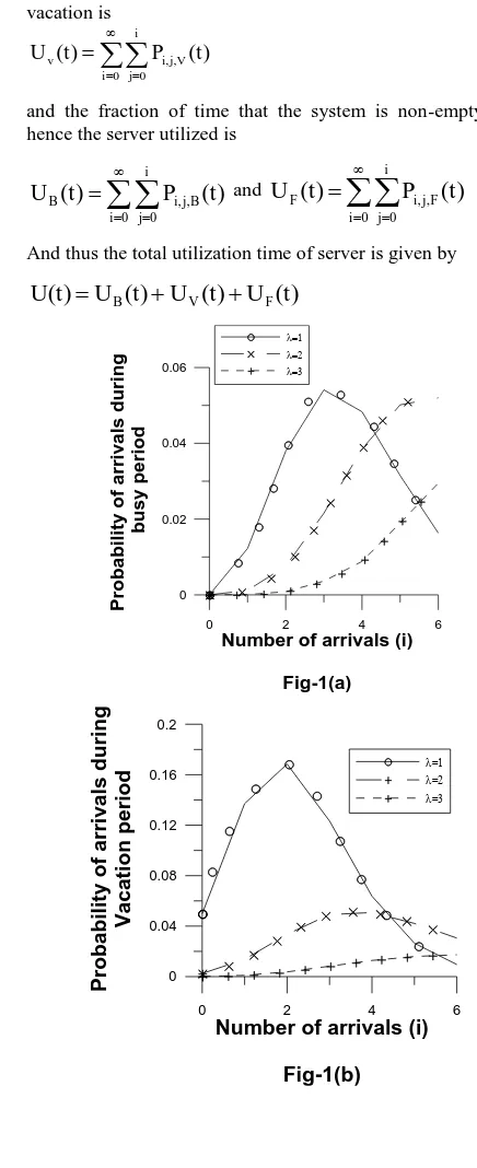
In this section, to demonstrate the efficiency of our analytical results we perform numerical experiment by using MATLAB. We study a special case of exponential service time during busy period, and probabilities of exact number of arrivals in the transient state are obtained.

The numerical result for the probabilities of exact number of arrivals

(i) by a given time i.e. i

i,j i,•

j 0

P (t)=P (t)





(ii) during busy period i.e.

i

i,j,B i,•,B

j 0

P

(t)

P

(t)







(iii) during working vacation period i.e.

i

i,j,V i,•,V

j 0

P (t)=P (t)





(iv) and during vacation

perio

d i.e. i

i,j,F i,•,F j=0

P (t)=P (t)



are computed for different sets of parameter and is summarized in Table – I. The Table – I shows complete agreement with the Table – I of Pegden & Rosenshine [7]. In addition, the columns having probabilities of arrivals during busy period, working vacation period and vacation period are obtained.

Table-I is based on the relationship

Pr {i arrivals in (0, t)} = i!

t) (λ eλt i₌





0 j

j i,(t)

P

where

P

i,j

(t)

is defined in eqn.(2.6).

Figure 1(a) to 1(d) indicates the changing curve

of_Pi,,B(t),

P

_i,,V

(t)

,

P

_{i, ,F}

(t)

and

P

_i,

(t)

with the increasing

of the arrival rate

λ

when the parameters

B V

μ



2,μ



1,w 1,.v=1and t 1





.

Table – I

w & v=1

λ

μB μV t i

i!

t)

(λ

e

λt i

=



 i

0 j

j

i,(t)

P



 i

0 j

B j ,

i, (t)

P



 i

0 j

V j ,

i, (t)

P



 i

0 j

F j ,

i, (t)

P

1 2 1 3 1 0.14936 1

0.012231 0.137130 0.0 1 2 1 3 3 0.22404

2

0.054104 0.123345 0.046592 1 2 1 3 5 0.10081

9

0.031480 0.026436 0.042903 2 2 1 3 1 0.01487

3

0.001218 0.013655 0.0 2 2 1 3 3 0.08923

5

0.021549 0.049128 0.018557 2 2 1 3 5 0.16062

3

0.050153 0.042118 0.068353 1 2 1 4 1 0.07326

3

0.004565 0.068697 0.0 1 2 1 4 3 0.19536

7

0.040020 0.123365 0.031982 1 2 1 4 5 0.15629

3

0.046405 0.046201 0.063688 2 2 1 4 3 0.02862

6

0.005864 0.018076 0.004686 2 2 1 4 5 0.09160

4

0.027198 0.027078 0.037327 2 4 2 4 5 0.09160

4

0.012199 0.053888 0.025516 1 2 1 4 4 0.19536

7

0.050982 0.087027 0.057358 1 2 1 3 6 0.05040

9

6. EXPRESSING VARIOUS

PERFORMANCE MEASURES

USING

P

i,j

(t)

6.1 The departure process from the M/M/1 queue has the distribution function

_P

_(t)

j ,

 , the probability that exactly j customers have been served by time t. In terms of_{P (t)}

j

i, , we have



 

 

j i

j i, j

,(t) P (t)

P &

(t) P (t) P (t) P (t)

P,j  ,j,B  ,j,V  ,j,F

where





  

j i

B j, i, B

j,

, (t) P (t)

P ,





  

j i

V j, i, V

j,

, (t) P (t)

P

and

_



  

j i

F j, i, F

j,

, (t) P (t)

P

Figs. 2(a) – 2(d) display the effect of different values of

λ

on

P

,j,B

(t),

P

,j,V

(t),

P

,j,F

(t)

&

P

,j

(t)

.

6.2 The probability of n customers in the system at time t, denoted by Pn(t)can be expressed in terms of

(t)

P

i,j as





  

0 j

j n, j n(t) P (t) P &

) t ( P (t) P (t) P (t)

P_n  _n,B  _n,V  _n,F

Where





 



0 j

B j, n, j B

n,

(t)

P

(t)

P

,





 



0 j

V j, n, j V

n,

(t)

P

(t)

P

&





 



0 j

F j, n, j F

n,

(t)

P

(t)

P

Figs. 3(a) – 3(d) depict the effect of different values of

λ

on

P

_n,B

(t),

P

_n,V

(t)

,

P

_n,F

(t)

&

P

_n

(t)

.

6.3 The waiting time distribution for a customer is defined as P(W>

τ

|t), the probability that a customer waits more than

τ

time units in the system, given that the customer arrives at time t, is given by



 

 

0 n

1) n τ by time services of

P(number Pn(t)

=

 

P

(t)

s!

μτ

e

_n

0 n

n 0 s

s μτ





  

Fig. 4 depicts waiting time for different values of

τ

. 6.4 The cumulative distribution for the sojourn time in the system is P(W



τ

|t) and the sojourn time is the waiting time plus the service time of a customer. Thus, we have

P(W



τ

|t) = 1-

 

P

(t)

s!

μτ

e

_n

0 n

n 0 s

s μτ





  

6.5 The system utilization, i.e. the fraction of time the server is busy until time t can also be expressed in terms of

P

i,j

(t)

. Thus the fraction of the time the

system is empty and consequently the server is on working vacation is



   

0 i

i

0 j

V j, i,

v(t) P (t)

U

and the fraction of time that the system is non-empty and hence the server utilized is





 



0 i

i

0 j

B j, i,

B

(t)

P

(t)

U

and





 



0 i

i

0 j

F j, i,

F

(t)

P

(t)

U

And thus the total utilization time of server is given by

(t)

U

(t)

U

(t)

U

U(t)



B



V



F

0 2 4 6

Number of arrivals (i) Fig-1(a)

0 0.02 0.04 0.06

P

ro

b

a

b

il

it

y

o

f

a

rr

iv

a

ls

d

u

ri

n

g

b

u

s

y

p

e

ri

o

d

  

0 2 4 6

Number of arrivals (i)

Fig-1(b)

0 0.04 0.08 0.12 0.16 0.2

P

ro

b

a

b

il

it

y

o

f

a

rr

iv

a

ls

d

u

ri

n

g

V

a

c

a

ti

o

n

p

e

ri

o

d 

0 2 4 6

Number of arrivals (i)

Fig-1(c)

0

0.02 0.04 0.06 0.08

P

ro

b

a

b

il

it

y

o

f

a

rr

iv

a

ls

d

u

ri

n

g

N

o

n

-E

x

h

a

u

s

ti

v

e

s

e

rv

ic

e _



0 2 4 6

Number of arrivals(i)

Fig-1(d)

0

0.05 0.1 0.15 0.2 0.25

P

ro

b

a

b

il

it

y

o

f

a

rr

iv

a

ls

  

0 1 2 3 4 5

Number of departures (j)

Fig-2(a)

0 0.02 0.04 0.06 0.08 0.1

P

ro

b

a

b

il

it

y

o

f

d

e

p

a

rt

u

re

s

d

u

ri

n

g

b

u

s

y

p

e

ri

o

d

  

0 2 4 6

Number of departures (j)

Fig-2(b)

0 0.04 0.08 0.12 0.16 0.2

P

ro

b

a

b

il

it

y

o

f

d

e

p

a

rt

u

re

s

d

u

ri

n

g

V

a

c

a

ti

o

n

p

e

ri

o

d

_



0 1 2 3 4 5

Number of departures (j)

Fig-2(c)

0

0.02 0.04 0.06 0.08 0.1

P

ro

b

a

b

il

it

y

o

f

d

e

p

a

rt

u

re

d

u

ri

n

g

N

o

n

-E

x

h

a

u

s

ti

v

e

S

e

rv

ic

e

  

0 2 4 6

Number of departures (j)

Fig-2(d)

0 0.1 0.2 0.3 0.4

P

ro

b

a

b

il

it

y

o

f

d

e

p

a

rt

u

re

s

  

0 2 4 6

Number of customers (n)

Fig-3(b)

0 0.1 0.2 0.3 0.4

P

ro

b

a

b

il

it

y

o

f

n

c

u

s

to

m

e

rs

d

u

ri

n

g

V

a

c

a

ti

o

n

p

e

ri

o

d



 

0 1 2 3 4 5

Number of customers (n) Fig-3(c)

0 0.02 0.04 0.06 0.08

P

ro

b

a

b

il

it

y

o

f

n

c

u

s

to

m

e

rs

d

u

ri

n

g

N

o

n

-E

x

h

a

u

s

ti

v

e

S

e

rv

ic

e

  

0 2 4 6

Number of customers (n)

Fig-3(d)

0 0.1 0.2 0.3 0.4

P

ro

b

a

b

il

it

y

o

f

n

c

u

s

to

m

e

rs

  

1 2 3 4 5 6

Time (

Fig-4 0

0.2 0.4 0.6 0.8

W

a

it

in

g

t

im

e

d

is

tr

ib

u

ti

o

n

Waiting time

6. CONCLUSION

The Two-dimensional state M/G/1 queueing system with working vacation and non-exhaustive service has been investigated. The numerical analysis clearly demonstrates the meaningful impact of the working vacations and non-exhaustive service on the system performances. The present investigation can be extended by incorporating bulk input/service.

7. REFERENCES

[1] Baba, Y., 2005. Analysis of a GI/M/1 queue with multiple working vacations. Oper. Res. Lett. 33, 201– 209.

[2] Hubbard, J.R., Pegden, C.D. and Rosenshine, M., 1986. The departure process for the M/M/1 queue, Journal of Applied Probability, Vol. 23, No. 1, pp.249-255.

[3] Indra, 1994. Some two-state single server queueing models with vacation or latest arrival run, Ph.D. thesis, Kurukshetra University, Kurukshetra.

[4] Indra and Ruchi, 2009. Transient Analysis of Two-Dimensional M/M/1 Queueing System with working vacations, Journal of Mathematics and System Science, Vol. 5, No. 2, pp. 110-128.

[5] Indra and Vijay, 2005. A two-state queueing model with intermittent available server and departures in batches of variable size, Vision 2020: The Strategic Role of Operational Research, Allied publishers, pp. 222-232.

0 2 4 6

Number of customers (n)

Fig-3(a)

0 0.02 0.04 0.06 0.08

P

ro

b

a

b

il

it

y

o

f

n

c

u

s

to

m

e

rs

d

u

ri

n

g

b

u

s

y

p

e

ri

o

d

[6] Kim, J.D., Choi, D.W., Chae, K.C, 2003. Analysis of queue-length distribution of the M/G/1 queue with working vacations In: Hawaii International Conference on Statistics and Related Fields.

[7] Pegden, C.D. and Rosenshine, M., 1982. Some new results for the M/M/1 queue, Mgt Sci Vol. 28, pp. 821-828.

[8] Servi, L.D. and Finn, S.G., 2002. M/M/1 queues with working vacations (M/M/1/WV), Performance Evaluation, Vol. 50, pp 41-52.

[9] Sharda and Indra, 1995. Explicit transient and steady state queue length probabilities of a queueing model with server on vacation providing service intermittently, Microelectronic Reliab. Vol. 35, No.1, pp-13-23.

[10]Takagi, H., 1991. Vacation and Priority Systems, Part 1. Queueing Analysis: A Foundation of Performance Evaluation, vol. 1. North-Holland/Elsevier, Amsterdam.

[11]Tian, N., Zhang, Z.G., 2006. Vacation Queueing Models: Theory and Applications. Springer, New York.