Available online at: www.ijcncs.org
E-ISSN 2308-9830 (Online) / ISSN 2410-0595 (Print)
Maintaining Water Surface Coverage by Mobile Sensor Nodes
with Energy Harvesting
Ryo Katsuma1 and Hirotaka Ueno2
1, 2
Graduate School of Science, Osaka Prefecture University
E-mail: 1ryo-k@mi.s.osakafu-u.ac.jp, 2st301006@edu.osakafu-u.ac.jp
ABSTRACT
Wireless sensor networks (WSNs) require long network lifetime and adequate field coverage, which can be problematic under certain conditions. Several studies have addressed these problems using energy harvesting or mobile sensor nodes. However, it is difficult to maintain field coverage on the surface of water for extended periods because of sensor node movement by water current. Therefore, a dynamic method to adjust the positions of sensor nodes is required. We propose a distributed algorithm to move sensor nodes dynamically and schedule node condition (active or sleeping) to maintain water surface field coverage for extended periods. Simulation results confirm that the features of proposed method can improve the duration of field coverage by 32%.
Keywords:Sensor Network, Mobile Sensor Node, Energy Harvesting, Coverage, Moving Schedule.
1 INTRODUCTION
In wireless sensor networks (WSNs), sensor nodes periodically sense, record, and transmit environmental information such as temperature and images. Recently, modern sensor devices are smaller, weightless, and demonstrate high performance. Consequently, sensor nodes can obtain a variety of information such as temperature, humidity, images, sound, light, and object motion. In WSNs, appropriate infrastructure is unnecessary because sensor nodes satisfy two roles; sensing and communication. We can employ WSN services even in places where it is difficult to deploy such infrastructures, e.g., on water. Therefore, sea monitoring WSNs have attracted significant attention for tsunami detection and fishery support [1][2]. One of the major problems of WSNs is extending network lifetime by energy-efficient mechanisms, which is referred to as the extend lifetime problem. A sensor node has limited battery power and must be recharged when the power is depleted. Conventionally, wired power supplies are employed to recharge batteries. However, wired power systems cannot be used in water-surface monitoring WSNs; thus, operating such WSNs for extended period is challenging. For example, it is difficult to recharge WSN node batteries when
measuring temperature at the surface of the sea; significant time and costs are required to retrieve, recharge, and redeploy such sensor nodes.
example, sensor nodes are moved by water current and wind in water-surface monitoring WSNs, and field coverage for such WSNs has been studied [7].
However, no study has attempted to solve the extend lifetime problem and coverage problem for water-surface monitoring WSNs simultaneously.
Herein, we target water surface WSNs for sea monitoring. Each sensor node has a solar panel that recharges its battery, and we use mobile sensor nodes to adjust node positions moved by water current and wind. A simple solution to operate WSNs for extended periods is to deploy a very large number of nodes. In this manner, some sensor nodes cover the entire area and others are put to sleep. Sleeping nodes can be initiated only as required, which conserves battery power. However, deploying a large number of nodes incurs huge cost. Our objective is to minimize the number of sensor nodes required to operate WSNs for extended periods. We propose an efficient method to schedule node condition (active or sleeping) and move nodes as required using a distributed algorithm.
We have implemented the proposed method as an algorithm and evaluated it by a simulation experi-ment compared to the algorithm whose part is invalidated. As a result, we have verified the effectiveness of the proposed scheme.
This study is organized as follows. In Section 2, we describe related work. Assumptions and target problem formulation are described in Section 3. The algorithm proposed to solve the target problem is described in Section 4. We evaluate the performance of the proposed method in Section 5 and present conclusions and suggestions for future work in Section 6.
2 RELATED WORK
There are two major problems with WSNs. The first problem is the extension of lifetime using energy efficient mechanisms. WSNs must be able to operate for extended periods. However, the lifetime of WSNs is limited because of finite battery power in sensor nodes. Several studies have attempted to address this problem using EH techniques.
Gilbert et al. introduced energy resources expect-ed to be usexpect-ed for energy harvesting techniques to transform resources into energy for WSNs. They also compared and discussed their features [8]. Steck et al. proposed SHiMmer, which is a system controller for a platform to manage EH techniques [9]. They discussed the change degree of energy harvest efficiency in changing environments. These studies have shown the usefulness of the EH
technique for WSNs. Ota et al. proposed a WSN lifetime extension method that estimates future battery charge for each node [10]. However, these studies targeted WSNs using static sensor nodes. A sensor node deployed on the sea surface moves constantly with water current and wind; therefore, the position of such nodes must be adjusted by a movement mechanism. An EH-based WSN lifetime extension method is required for mobile sensor nodes that consume energy rapidly by adjusting their positions.
The second problem is adequate coverage of the field of interest using the minimal number of active sensor nodes. Several studies have examined adequate field coverage using mobile sensor nodes. Methods to maintain adequate field coverage must consider both node positions and energy consump-tion in mobile nodes.
Wang et al. proposed a field coverage method using mobile nodes that move only once to save energy [6]. However, it is difficult to adapt to changing environments such as water currents and wind. Mobile nodes must be able to move to appropriate positions periodically. Luo et al. proposed a water current model and a method to cover a lake surface field using mobile nodes [7]. Their water current model represents uncontrollable movement of sensor nodes on the water surface. These methods can extend the lifetime of WSNs by balancing the energy consumption of each node. However, such methods assume that the battery of each mobile node cannot be recharged.
These existing studies have attempted to solve either the extend lifetime problem using EH or the coverage problem for mobile WSNs. To the best of our knowledge, no study has attempted to address these problems simultaneously. In this study, we propose a method to maintain field coverage for extended periods using a minimal number of mobile nodes with energy recharge units.
3 PROBLEM FORMULATION
Here, we describe the assumptions and the probl-em formulation.
3.1 WSN Assumptions
We target water-surface monitoring WSNs, such as those employed to find fish, and provide beach security for swimmers. A sensing field on the sea surface must be covered by active sensor nodes, and such nodes move by water current and wind.
communication range are denoted as Rs and Rc,
respectively. A sensor node has two operating modes, i.e., active and sleep modes. Active nodes sense environmental data each period I and send the data to a sink node via multi-hop communication. In the proposed method, we assume that no objects intercept radio waves; thus, each node can send packets via multi-hop communication. Multi-hop communication has low energy requirements and demonstrates high qualityof service [11]. An active node can move to a destination using the equipped motor and screw. In addition, to conserve energy, sleeping nodes cease most operations. We wake a sleeping node by sending a wakeup signal as required. A sleeping node can also charge its battery using solar power generation. We use the Carrier Sense Multiple Access/Collision Avoidance protocol for node communication to avoid radio interference. Note that a sensor node consumes energy by sensing, communicating, and moving. We define the energy consumption model in Subsection 3.2.
3.2 Energy Consumption Definitions
A sensor node has finite battery and it is not feasible to physically replace the battery upon exhaustion. The initial energy and maximum energy for each sensor node are denoted Einit, and E,
respectively.
A sensor node consumes energy by sensing, transmitting, and receiving data. Consumed power for sensing x[bit] data Sens(x) is expressed by Formula (1).
sens elecx E E
x)
(
Sens (1)
Here, Esens and Eelec are constant values that
represent the power required by sensing and information processing, respectively.
Consumed power Esens is a constant value.
Consumed powers Trans(x, d) and Recep(x) required to transmit x[bit] for d[m] and receive x[bit] are expressed by Formulas (1) and (2), respectively [12].
2 )
, (
Trans x d Eelecxampxd (2)
x E d
x, ) elec
(
Recep (3)
Here, amp is a constant value that represents the
power required by amplification.
Consumed power Move(d) required to move d
[m] is expressed by Formula (3) [3].
move E d
d)
(
Move (4)
Here, Emove is a constant value that represents the
power required to move a node by a distance of 1[m]. A sleeping node can charge its battery using solar power generation. The amount of solar power generated depends on the intensity of solar radiation, which varies according to changing environmental conditions. We denote the intensity of solar radiation at night, during a cloudy day, and during a sunny day as cnight(t), ccloudy(t), and csunny(t),
respectively. The amount of solar power generated at solar radiation intensity c([t, t+u]) from t to t+u
seconds is expressed by Formula (4).
]) , ([ ])) , ([ , (
Csolar u c t t u
chargeuc t tu (5)Here, charge is the coefficient for the amount of
energy charged per unit time.c([t, t+u]) conforms Formula (6). k j i kc jc ic u t t c
]) night cloudy sunny ,
([ (6)
Here, i, j, and k are the rates of night, cloudy, and sunny time during [t, t + u], respectively.
3.3 Problem Formulation
The inputs for the target problem are target field, initial sensor node battery power, sensing range,
constant values Esens, Eelec, Emove, amp, and expected
WSN operation time T. The outputs are the number of sensor nodes, the destination point of each node for each time t, and the operating mode of each sensor node (active or sleeping). We refer to this set of outputs as the node schedule.
Note that the field must always be covered by active sensor nodes for the expected period T. Following Formula (7) represents this condition.
1 ) , ( , ,
pos Field t T Cover post (7)
Here, Cover(pos, t) is the number of active nodes covering the point pos at time t.
0 ])) | ) ( . ) ( . | , ([ ( |) ) ( . ) ( . (| Move ) ( . ,
solar
v t pos s t dest s t t c C t pos s t dest s t energy s T t (8)
Here, T, v and |s.dest(t)-s.pos(t)| represent the expected WSN operation time, the speed of a mobile node and the moving distance, respectively.
If some sensor nodes operate for extended periods, their energy will be exhausted and the WSN will not be able to maintain field coverage. The goal of this study is to minimize the number of sensor nodes n
that satisfy the condition expressed by Formulas (7) and (8). The objective function is shown in Formula (9).
)
(
minimize
n
(9)3.4 Approach
To solve the target problem, we determine a set of active and sleeping nodes, as well as the destination of each sensor node, simultaneously. Note that there are many destination candidates for each sensor node; thus, it is difficult to determine the specific destination for each sensor node that would result is low energy consumption when the node in question is moved and thus satisfies the condition expressed by Formula (7).
To simplify this problem, we set sensing points
on the field in a grid spacing of 2Rs and assign a unique ID to each sensing point. If active nodes with sensing range radius Rs are deployed at all sensing points, the field is covered. Initially, we deploy k nodes and determine a single active node of k nodes for each sensing point. Note that the method proposed in Section 4 periodically adjusts the position of each sensor node that is moved by water current.
Fig. 1. Example of effective exchange.
Sensor nodes are provided with the node number and coordinates of the sensing point that they belong to, and the proposed method ensure that these nodes return to the specified sensing points upon displacement by water current or wind to maintain field coverage. The proposed method also equalizes the residual battery power of each sensor node by appropriate exchange of two sensor nodes belonging to different sensing points.
4 PROPOSED METHOD
Here, we explain the proposed algorithm to solve the problem defined in Section 3. The proposed algorithm determines the node destinations and the node operating mode schedules to maintain field coverage for extended periods by equalizing the residual battery power of each node.
For example, for sensing points P and Q, sensor nodes p1 and q1 belong to P and Q, respectively.
Nodes p1 and q1 are moved by water current, as
shown in Fig. 1. When p1 and q1 must return to
sensing points, it is better to exchange their destinations (Fig. 1(b)) because each node will then have to move a shorter distance and thus will consume less energy compared with the case when returning to the original positions. We propose an algorithm to exchange the sensing points of two sensor nodes for energy efficient adjustment of node position.
4.1 Action Conditions of Algorithm
Initially, k sensor nodes are deployed at each sensing point. For each sensing point, the youngest sensor node ID of nodes belonging to the same sensing point begins sensing environmental information and other nodes are set to sleep. The proposed algorithm, which determines sleep scheduling and node destinations, runs when at least one of the following three conditions is satisfied. Active node s judges the conditions by periodically communicating with the other nodes belonging to the same sensing point.
α
) a time I since the WSN starts elapses or the proposed algorithm finishesβ
) residual battery power of a node s decreases to 1/p (p is constant value) of the maximum battery power of other nodesγ
) distance between s and s.sp.pos increases, and the following formula (10) is satisfiedc t v pos sp s pos s range s | . . . |
Here, s.range is the radius of the sensing range centered on the sensing point to which s belongs,
s.pos are the coordinates of s, and s.sp.pos are the coordinates of the sensing point to which s belongs.
tc is the expected total calculation time of the
proposed algorithm, which is expressed by Formula (11).
2 2t t
tc i (11)
Here, t1 is the time required to collect information
on the coordinates and residual battery power of other nodes, and t2 is the calculation time of the
proposed algorithm.
For condition
α
, we adjust the position of sensor nodes moved by water current periodically. Forcondition
β
, a sensing node consumes its battery power by sensing, and the proposed algorithm changes the set of sensing nodes to achieve equalization of residual battery power among all nodes. For conditionγ
, if a sensing node moves away from its sensing point, the field coverage may not be satisfied. The proposed algorithm determines a new set of sensing nodes before a sensing node is carried away by a current.4.2 Destination Decision Algorithm
In this subsection, we describe the proposed algorithm performed by sensing node s to determine satisfaction of one or more of the conditions presented in Subsection 4.1. Here, s.sp
denotes the sensing point to which s belongs, and Z
is a set of sensor nodes belonging to s.sp.
1. s collects the residual battery power and position of each node in Z via multi-hop communication using the On Demand Distance Vector routing protocol.
2. Using Formula (3), s predicts the residual battery power of all sensor nodes in Z after they move from their current positions to
s.sp.pos.
3. s selects node p whose residual battery Ep is the maximum residual battery power among nodes calculated in step (2). s executes the
belonging exchange algorithm (explained in Subsection 4.3) for node p.
4. If p’s sensing point is exchanged with a node (e.g., node q) in step (3), s sets the destination
p.sp.pos to p (i.e., it returns to p’s new sensing point) and q.sp.pos (= s.sp.pos) to q. Otherwise, the destination of p if set to
s.sp.pos.
If full-battery nodes belonging to s.sp exist in Z
(with the exception of p and q), then the node s
commands them to move straightly toward s.sp.pos
until they consume l% of their battery power (l is a constant).
4.3 Belonging-Exchange Algorithm
Here, assume that sensor node p is moved by water current and wind. Note that p may approach another sensing point. When there are two such nodes p and q, nodes consume less energy by moving to the nearest sensing point. In this section, we present an algorithm to exchange sensing points to which such nodes belong in order to facilitate extended WSN operation. This proposed algorithm runs in the destination decision algorithm described in Subsection 4.2. Here, each notation is the same as those presented in Section 4.2.
1. Sensing node s communicates with sensing node b belonging to B, which is the nearest sensing point to p, and requires b to send the node information (i.e., residual battery power and positions of all nodes belonging to b.sp).
2. b wakes up other nodes belonging to b.sp
wake up temporarily and obtains their residual battery power information and co-ordinates.
3. b finds a node q with the maximum residual battery of nodes belonging to b.sp and sends the battery power and position information to
s.
4. s predicts the residual battery power Eq of q
when q move to s.sp.pos.
5. Each sensing point of p and q is exchanged if
(a) Position example before applying algorithm.
(b) Prediction of residual batteries.
(c) Applied case of exchange algorithm.
Fig. 2. Algorithm application.
An example exchange performed by this algorithm is shown in Fig. 2. Here, consider two sensing points A and B. In Fig. 2, we show sensing points (circles), nodes (squares), and show residual battery power. a1, a2, a3, and a4 are sensor nodes
belonging to A, and b1, b2, b3, and b4 are sensor
nodes belonging to B. Now consider a case in which nodes a4 and b4 have approached sensing
points B and A, respectively. Assume that sensing node a1 at sensing point A satisfies a condition of the algorithm and begins calculations (Fig. 2(a)). In Fig. 2(b), a1 collects information about the residual
battery power and the position of each node belonging to A and identifies a4 as the candidate for
the next sensing node at A. Here, the sensing point closest to a4 is B. a1 communicates with node b1
(sensing at B) and obtains information from b1
about residual battery power and the position of each node belonging to B. a1 predicts residual
battery power after nodes belonging to B have moved to A. In this case, the residual battery power of b4 is greater than that of a4, b1, b2, and b3 (Fig. 2(c)). Therefore, the sensing points of a4 and b4 are exchanged.
5 PERFORMANCE EVALUATION
5.1 Experimental Settings
In this section, we describe simulation results of an evaluation of the proposed method.
In water-surface monitoring WSNs, water current and wind move sensor nodes. We improve an existing water current model [7] by adding wind influence.
We performed computer simulations to measure the field coverage time that the proposed method can maintain by varying the number of deployed sensor nodes. In order to evaluate the effect of the proposed features, we compared the proposed method with three methods. No-exchange method is the proposed method whose belonging-exchange mechanism is invalidated. No-prediction method is the proposed method without predicting the residual battery amount after moving. No-prediction method also applies the belonging-exchange mechanism such that the total moving distance of nodes is minimized. No-generation method is the proposed method whose energy harvesting mechanism is invalidated. We used a desktop computer with an Intel Core2Duo U9600 (1.60 GHz) CPU, 2 GB memory, Windows 7 Professional, and All-In-One Eclipse 3.1 for the simulations.
5.2 Water Current Model
The existing water current model [7] represents a lake surface without wind. We have added wind influence to this model for our simulations. Generally, water current tends to flow in a certain direction (referred to as the main-flow model). Changes in wind direction are more random than changes in water current direction (referred to as the random-flow model). Therefore, we combine both main- and random-flow model.
5.3 Simulation Result
In our simulation, we deployed 27-585 sensor
nodes on an 84 [m]
×
84 [m] field. The sensing radius of a sensor node is 20 [m]. The distance between sensing points is approximately 28 [m], and the number of sensing points is 9 (Subsection 3.4). Sensor nodes sense environmental information every 30 min. The initial maximum battery power is 32400 [J] (comparable to two AA batteries). The energy consumption coefficient for data processingEelec is 50 [nJ/bit] [13]. The energy consumption
coefficient for signal amplification amp is 100
[pJ/bit/m2] [13]. The energy consumption for sensing and moving are 0.018 [W] and 5.6 [W/m], respectively. The communicable range Rc is 100
[m]. Parameters p and tc shown in Subsection 4.1
are set to 2 and 1, respectively. Parameter l shown in Subsection 4.2 is set to 30%. Each sensor node can communicate with almost other nodes over a single hop. Even if sensing node cannot obtain the information of other nodes’ residual battery power, the proposed algorithm can run by using only obtained information. However, in this case, the performance of the proposed algorithm may drop. Communication time t1 is a sufficiently small.
According to results obtained in the preliminary experiments, the calculation time of the proposed algorithm is approximately 2000 ns. Note that the proposed algorithm ignores the calculation time t2.
Fig. 3. WSN lifetime (main-flow speed is less than 0.5[m/s]).
Fig. 4. WSN lifetime (main-flow speed is less than 0.3[m/s]).
Fig. 5. WSN lifetime (main-flow speed is less than 0.1[m/s]).
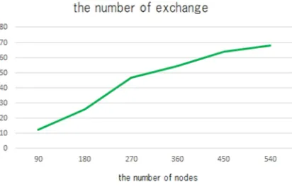
Fig. 4. the number of belonging-exchange.
Fig. 4 shows the number of belonging-exchange. We can see the linear increase like the operation lifetime. This is one of evidence for the proposed mechanism extends the lifetime.
We also conducted simulations for rapid water current. However, each number of nodes maintains similar lifetime. The reason for the similar values is that as water current and wind move sensor nodes, sensor nodes consume significantly more energy to adjust their positions than energy consumed for only sensing and communication. Furthermore, WSN lifetime can be extended on a field with less influence from water current and wind.
6 CONCLUSION
In this study, we have formulated a time coverage problem for water-surface monitoring WSNs. We have proposed a method to address this problem by setting sensing points and exchanging the points to which sensor nodes belong. Simulation results have confirmed that the proposed features improve WSN operation time.
Near future, we plan to improve the proposed method for long-term WSN operation (one month or greater). For example, we could employ anchors to avoid sensor node movement resulting from water current and wind. In addition, we plan to investigate the use of a low-cost infrastructure in our target problem and proposed algorithm.
7 REFERENCES
[1] Casey, K., Lim, A. and Dozier, G., “A Sensor Network Architecture for Tsunami Detection and Response”, ACM Int’l. J. of Distributed Sensor Networks - Selected Papers in Innovations and Real-Time Applications of Distributed Sensor Networks, Vol. 4, No. 1, 2008, pp. 28-43.
[2] Alkandari, A., Alnasheet, M., Alabduljader, Y. and Moein, S. M., “Wireless Sensor Network (WSN) for Water Monitoring System: Case Study of Kuwait Beaches”, Proceedings of Digital Information Processing and Communications (Klaipeda), July 10-12, 2012, pp. 10-15.
[3] Rahimi, M., Shar, H., Sukhatme, G., Heideman, J. and Estrin, D., “Studying the Feasibility of Energy Harvesting in a Mobile Sensor Network”, Proceedings of Robotics and Automation (Taipei), September 15-18, 2003, pp. 19-24.
[4] Kansal, A., Hsu, J., Zahedi, S., and Srivastava, M. B., “Power management in energy harvesting sensor networks”, ACM Trans. On Embedded Computing Systems (TECS) - Special Section LCTES’05, 2007, Article No. 32.
[5] Luo, R.C., and Chen, O., “Mobile Sensor Node Deployment and Asynchronous Power Man-agement for Wireless Sensor Networks”, IEEE Trans. on Industrial Electronics, Vol. 59, Issue 5, 2011, pp. 2377-2385.
[6] Wang, Y. C., and Tseng, Y. C., “Distributed Deployment Schemes for Mobile Wireless Sensor Networks to Ensure Multi-level Coverage”, IEEE Trans. on Parallel and Distributed Systems, Vol. 19, No. 9, 2007, pp. 1280-1294.
[7] Luo, J., Wang, D. and Zhang, Q., “Double Mobility: Coverage of the Sea Surface with Mobile Sensor Networks”, Proceedings of International Conference on IEEE INFOCOM, (Rio de Janeiro), April 19-25, 2009, pp. 118-126.
[8] Gilbert, M., J., and Balouchi, F., “Comparison of Energy Harvesting Systems for Wireless Sensor Networks”, Int'l J. of Automation and Computing, 2007, pp. 334–347.
[9] Steck, B., J., and Rosing, S., T., “Adapting Performance in Energy Harvesting Wireless Sensor Networks for Structural Health Monitoring Applications”, Proceedings of Int'l Workshop on Structural Health Monitoring (Stanford University), September 9-11, 2009, pp. 118-126.
[10]Ota, K., Kobayashi, K., Yamazato, T., and Katayama, M., “Relay Selection Scheme with Harvested Solar Energy Prediction for Solar-Powered Wireless Sensor Networks”, IPSJ SIG
Mobile Computing and Ubiquitous
Communications (2012-MBL-61), Vol. 31, 2012, pp. 1-8.
Networks Using Mobile Relays”, IEEE Communications Magazine, Vol. 51, No. 7, 2013, pp. 122-129.
[12]Heinzelman, W.R., Chandrakasan, A., and Balakrishnan, H., “Energy-efficient communication protocol for wireless microsensor networks”, Proceedings of the 33rd Hawaii Int'l. Conf. on System Sciences (Hawaii), January 4-7, 2000, pp. 1-10.
[13]Wang, G., Cao, G., La Porta, T., and Zhang, W., “Sensor Relocation in Mobile Sensor Networks”, Proceedings of International Conference on IEEE INFOCOM, (Miami), March 13-17, 2005, pp. 2302-2312.
AUTHOR PROFILES:
Ryo Katsuma received a bachelor’s degree in education from Kyoto University of Education in 2006. He also received master’s and doctoral degrees in engineering from the Nara Institute of Science and Technology. He is currently an assistant professor at Osaka Prefecture University. His research field of interest is ad-hoc networks.


![Fig. 4. WSN lifetime (main-flow speed is less than 0.3[m/s]).](https://thumb-us.123doks.com/thumbv2/123dok_us/1327509.1640925/7.612.319.544.97.223/fig-wsn-lifetime-main-flow-speed-m-s.webp)