Abstract— In this paper, internal multi-model control method to the case of nonlinear discrete-time systems is proposed. This control approach is based firstly on the method of switching between different partial commands and secondly on residues techniques. We are interested in this article to the affine control nonlinear systems. The nonlinear system can be described by a library of linear models. We use the multi-model approach to determinate the internal multi-models of this control structures. To validate this method, simulation results are presented.
Index Term— Internal multi-model control IMMC,
non-linear systems, affine non-non-linear control systems, switching method, residues techniques.
I. INTRODUCTION
The multi-model approach is a mathematical approach that represents the best possible the dynamic operation of a nonlinear process, using Linear models time-invariant (LTI). The non-linear problems interest the mathematicians and physicists because most physical systems are nonlinear. A non-linear system is a set of equations (differential, for example) nonlinear, describing the temporal evolution of the constituent variables of the system under the action of a finite number of independent variables called input or control variables, or simply commands that can freely choose, to realize certain objectives.
Several classes of nonlinear systems are evoked in the literature such as the affine nonlinear control systems, we will propose to focus on this class of systems in this paper.
Robustness has become a desirable quality of the solutions for the control problems. Robustness of a system is defined by the invariance of some qualitative properties of the system such as stability and performance against the environmental disturbances and model uncertainties.
Many control techniques have been developed to solve this problem, we can mention the sliding mode control, the H∞ control approach and the internal model control method. This internal model control strategy is generally used because of its robustness, it comprises an explicit internal process model and a controller. [7,10]
In this paper, we propose to apply internal multi-model control approach for the case of discretized nonlinear systems.
We use a specific approach to the discretization of this class of nonlinear systems, the affine nonlinear control systems. This class of systems is particularly important for applications
industrial automation. We operate multi-model approach for the determination of internal models of this control structure.
This internal multi-model control approach is based firstly on the switching method of partial commands and secondly on the fusion method operating the residues techniques. [10]
In these control structures, synthesis of the controller is reduced to a problem of internal models inverse construction.[1] In addition, the direct inversion of the models is often impossible. Thus, the proposed controller synthesis approach is based on a specific inversion method. This approach has been modified to improve the accuracy of the controlled system. [8, 10, 11]
II. NON-LINEAR SYSTEMS
Nonlinear problems interest the engineers, physicists and mathematicians and many other scientists because most systems are inherently nonlinear in nature.
By definition, a non-linear system is a system which is not linear, that is to say (in the physical sense) which can not be described by linear differential equations with constant coefficients.
This definition, or rather non-definition explains the complexity and diversity of non-linear systems and methods that apply. There is not a general theory for these systems, but several methods suitable for some classes of nonlinear systems.
We will limit ourselves in this paper in the study of the affine nonlinear control systems.
Most physical systems have a nonlinear behavior. Nonlinear systems are more difficult to study than the linear systems, therefore this systems are commonly approximated by linear equations. Thus, by linearizing when possible a nonlinear system around an equilibrium point, we obtain a linear system that correctly represents the nonlinear system in the vicinity of this equilibrium point.
Nonlinearities can be of different types:
Non linearity natural (physical systems): These nonlinearities often induce undesirable effects
No artificial linearity (control systems) are implemented in order to offset the effects induced by the natural nonlinearities
The systems that we are studying in this article are the affine nonlinear control systems.
Internal Multi - Model Control of Non-linear
Discrete-time Systems
Chakra Othman
1, Dhaou Soudani
21,2Automatic Research Laboratory. L.A.R.A, National Engineering School of Tunis (ENIT), Tunis El Manar
University, Tunis, Tunisia
III. DISCRETIZATION OF NONLINEAR SYSTEMS
We are interested in this article to the affine nonlinear control systems. This type of systems is defined by a state space representation of the form:
.
( )
( ) ( )
( )
( ) ( )
X
A X X
B X U t
Y
C X X
D x U t
(1)where
U
mis the input of the system,X
nthe state of the system,Y
pthe system output.There are many methods to discretize a nonlinear affine control system which are inspired from the approximation principle method of the continuous systems.
We consider the following polynomial form that represents an approximation of the affine nonlinear control systems: [3]
.
[ ] [ 1]
1 1
(
(
))
r r
i j
i j n
i j
X
A X
B I
X
U
(2)with : [ ] 1
( )
r i i iA X
A X
[ 1] 1( )
(
)
r j j n jB X
B I
X
The desired discrete model must also have a polynomial affine structure of the form: [8]
[ ] [ 1]
1
1 1
(
(
))
r r
i j
k i k j n k k
i j
X
E X
F I
X
U
(3)We are interested in a discretization approach for nonlinear affine control systems to characterize a discrete system from an affine continuous system. This discretization approach is based on the following approximation: [4,13]
for t[kT, (k+1)T[ :
1 . 1 [ ] [ ]
( )
2
( )
( )
;
2
( )
k k k k i i k kX
X
X t
X
X
X t
T
X
t
X
i
U t
U
(4)This approximation leads us to the following discrete equation:[4,13]
[ ] [ 1]
1
1 1
(
(
))
r r
i j
k i k j n k k
i j
X
E X
F I
X
U
(5)with : 1 1 1 1 1 1 1 1
2
2
;
2
2
;
1
2
n n n i i n i iI
A
I
A
E
T
T
I
A
E
A i
T
I
A
F
B i
T
IV. INTERNAL MODEL CONTROL STRUCTURE
The internal model control method is known by its robustness, this control structure allows us to take into account the effects of modeling errors and external disturbances. [1, 2]
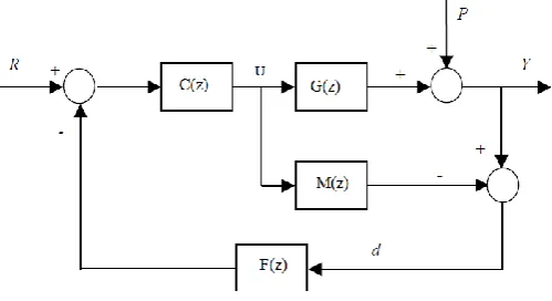
The internal model control structure comprises an internal model „M‟ which is an explicit model of the process to be controlled, a controller „C‟ which can be chosen the opposite of this model and a robustness filter „F‟. „P‟ is an additive disturbance on the output of the process.
In the basic structure of the IMC, the command signal „U‟ outcome from the corrector „C‟ is applied simultaneously to the process „G‟ and its model „M‟. The IMC exploits the behavior gap to correct the error on the reference. The error signal includes the influence of external disturbances and modeling errors.
We consider the basic structure of internal model control:
Fig. 1. Structure of the internal model control
with:
„R‟, „d‟, „Y‟ are respectively the reference to reach, the modeling error and the system output
Generally the internal model control structure includes a robustness filter usually introduced in the feedback loop. Its role is to introduce a certain robustness against the modeling errors.
In this article, we do not take into account the presence of the filter.
In the case where the controller of this control structure is chosen the inverse of the model, the error between the process output and its reference is asymptotically null, whatever the modeling error. Therefore the proposed regulator is the inverse of the model „M‟, if feasible, which requires the study of the realization of the model inverse.
In addition, the direct inversion of the model is often impossible. We proposed used an implementation method of the approximated inverse for systems with a transfer function whose order of the numerator is less than the order of the denominator, non-minimum phase systems and delay systems.
We consider the following diagram with „M(z)‟ is the model transfer function and „A1‟ is a gain to choose.[8,10,11]
Fig. 2. Basic idea to obtain the approximated inverse
The global transfer function of the scheme (2) is:
1
1
( )
1
( )
A
C z
A M z
(6) For sufficiently high values of the gain A1, the filter C(z)approaches the inverse of M(z) :
1
( )
( )
C z
M z
(7) Thus, the global transfer function C(z) is the approximated inverse of the model transfer function M(z).For some classes of systems such as non-minimum phase systems, delay systems, ... the gain A1 that ensures stability
of the loop that realize the filter C(z) may not be very high, which does not allow us to obtain the approximated inverse, therefore, we add a gain A2 to ensure a null static error. Thus,
a second structure of the corrector is proposed:
Fig. 3. structure of the second corrector used
The gain A2 is used to ensure the desired accuracy, it is
described by the following expression:
1 2
1
1
(1)
(1)
A M
A
A M
(8)V. INTERNAL MULTI-MODEL CONTROL STRUCTURE
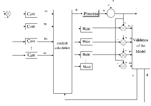
The multi-model represents nonlinear systems as a linear interpolation between in general local linear or affine models. Each local model is a dynamic system LTI (Linear Time Invariant) valid around an operating point. In practice, these models are obtained by identification, linearization around different operating points or convex poly-topical transformation.
The multi-model approach consists in representing the non-linear process by a set of linear models forming a library of templates. These linear models are at the origin of the elaboration of a new control structure called internal multi-model control structure denoted IMMC. By combining the internal model control structure and the multi-model approach, we obtain an internal multi-model control approach.
The internal multi-model control structure for nonlinear discrete-time systems was developed from the first one which is the internal model control. It considers as internal model the linear models library obtained from the nonlinear process. In this paper, we exploit the multi-model approach for obtaining local linear models of the nonlinear discretized system.
Considering the schema of the internal multi-model control structure: [2,3,9,10]
Fig. 4. Basic internal multi-model control structure of the discretized nonlinear systems
In this basic structure G (z) is the transfer function of the process to be controlled, M1(z), M2(z), M3(z),…,Mh(z) are
the transfer functions of the internal models, C1(z),C2(z),C3(z),…,Ch(z) are the transfer functions of the
controllers and v, d are respectively, the validation index of the nearest model and the modeling error.
In this control structure Mi(z) for i = 1,...,h are the linear
models library inspired from the non-linear process, „d‟ is the modeling error and „v‟ is the validation index.[5,10]
The proposed regulators for this control structure are the Mi-1 inverse models library that represents the inverse of the
internal models Mi.
There are several fusion methods on which are based multi-model structures.
We focus in this paper firstly, to the method of switching between different internal models and secondly to the fusion method based on residues techniques.
VI. INTERNAL MULTI-MODEL CONTROL APPROACH OF DISCRETIZED NONLINEAR SYSTEMS
A. First internal multi-model control structure based on switching method for non-linear discrete-time systems:
Fig. 5. Schema of the first internal multi-model control structure for non-linear discrete-time systems
A1,A2,A3,…,Ah are the gains used for the controllers
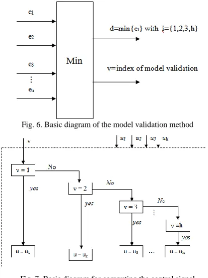
Among the different models, we choose the model that presents the slightest error. The chosen controller is then obtained from the model whose output is closest to the process, the validation block ensure the choice of this model. The figures (6) and (7) represent respectively the block diagram of the model validation method and the diagram describing the principle of control computation. [2,3,9,10]
Fig. 6. Basic diagram of the model validation method
Fig. 7. Basic diagram for computing the control signal
For some classes of systems, the gain Ai for i[1,..h] that
ensures stability of the loop that realize the filter Ci(z), may
not be very high, which does not allow us to obtain the approximated inverse, therefore, we add a gain A2i to ensure
a null static error. Thus, the second method to the realization of the approximated inverse is used. [8] A second internal multi-model control structure based on the switching principle is obtained:
Fig. 8. Diagram of the second internal multi-model control structure of the non-linear discrete-time systems
B. Second internal multi-model control structure based on the residues techniques method for non-linear discrete-time systems:
This internal multi-model control structure is based on residues techniques. Using the first realization method of the model inverse [8], this first internal multi-model control approach based on residues techniques is obtained:
Fig. 9. First diagram of the internal multi-model control structure for non-linear discrete-time systems based on residues techniques
The calculation of the global command to apply to the system depends on partial control signals related to models Mi for i=1,…,q and on the validity of models.[3,9,10]
Validity indices are inversely proportional to the difference between the system output and the outputs of the internal models that can be defined by:
( )
( )
( )
i i
d t
y t
y t
for i=1,..,h (9) We can express the validity by this expression:4
1
1
1
i i
j j
d
v
d
(10)
Thus, the global control signal can be defined by the following expression:
4
1
( )
i( ) ( )
ii
u t
v t u t
Using the second method described previously for the realization of the models inverse, we can obtain the following internal multi-model control structures:
Fig. 10. Second diagram of the internal multi-model control structure for non-linear discrete-time systems based on residues techniques
VII.APPLICATION
We consider the affine nonlinear control system defined by the following expression:
.
2
2
2
X
X
X
U
XU
(12) With:U: is the system input X: is the output of the system
We use the approach described above for the discretization of the nonlinear system with a sampling period T=0.1s. We obtain the following discrete nonlinear system:[3]
2
(
1)
0.81 ( ) 0.09
( ) 0.18 ( )
0.09 ( ) ( )
X k
X k
X
k
U k
X k U k
(13)Applying the Z-transform, we can obtain the following expression:
( )
0.18 0.09 ( )
( )
0.81 0.09 ( )
X z
X z
U z
z
X z
(14)We pose k1 and k2 such as:
1
0.18 0.09 ( )
k
X z
(15)2
0.81 0.09 ( )
k
X z
(16) We can obtain the following transfer function of the nonlinear discrete time system:1
2
( )
K
X z
z
K
(17) The system is stable for the state values of 0<X<2.11, subsequently, it is considered the variation of the system for X ranging from 0 to 2:for X=0 =>
k
1
0.18
k
2
0.81
for X=1 =>
k
1
0.27
k
2
0.9
We can represent the nonlinear system by the following four discrete linear local models:
( )
0.18
( )
0.81
X z
U z
z
(18)( )
0.18
( )
0.9
X z
U z
z
(19)( )
0.27
( )
0.81
X z
U z
z
(20)( )
0.27
( )
0.9
X z
U z
z
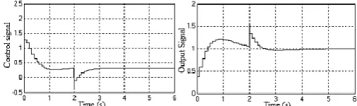
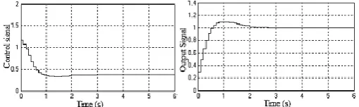
(21) For a unit step reference applied at k=0T, the simulation results by applying the first internal multi-model control structure based on the switching method for Ai=1 for i=1,..,4are denoted in the figure (11):
Fig. 11. Evolution of the control and output signals for Ai=1 for i=1,..,4
From figure (11), we notice that the static error is not null, this is because the gains Ai for i=1,..,4 that ensure
stability of the loop that realize the filter C(z) are not very high, which does not allow us to obtain the approximated inverses, thus, we add a gains A2i for i=1,..,4 to ensure a null
static error. So we decide apply the second multi-model control structure based on the switching technique which is presented in figure (8).
For the same reference, the simulation results for Ai=1
for i=1,..,4 and for A21=2.06, A22=1.55, A23=1.7 and
A24=1.37 are shown in the figure (12):
Fig. 12. Evolution of the control and output signals for Ai=1, A21=2.06, A22=1.55, A23=1.7 and A24=1.37 for i=1,…,4
From figure (12), we note that the system output has an overshoot on startup then it joins the reference.
The simulation results for Ai=1, A21=2.06, A22=1.55,
A23=1.7, and A24=1.37 for i=1,…,4 and by adding a
Figure 13: Evolution of the control and output signals in the case of the presence of a disturbance in the form of a step with amplitude of 0.5 which
appears at k=20T
From figure (13), we remark that this control structure allows us to reject the disturbance.
For the same reference and for a sampling period T=1s, the simulation results for the same values of the gains Ai and
A2i, for i=1,..,4 are indicated in the figure (14):
Fig. 14. Evolution of the control and output signals for a sampling period T=1s and for Ai=1, A21=2.06, A22=1.55, A23=1.7 and A24=1.37, for i = 1..4
Form figure (14), we notice that the system takes a longer time to stabilize compared to the system discretized with a period ten times smaller. We conclude that a high value of the sampling period can result in system instability.
Satisfactory results have been obtained using the second internal multi-model control approach based on the principle of the switching.
We now propose to apply the internal multi-model control approach that exploits the fusion method based on residues techniques. The Simulation parameters for residues techniques are taken the same as the switching method.
For the same reference, the simulation results with the first internal multi-model control structure based on residues techniques presented in figure (9) for Ai=1 for i =1,..,4 are
presented in figure (15):
Fig. 15. Evolution of the control and output signals for Ai=1 for i=1,..,4
It is noted that the output of the system does not follow the reference adequately, there are static errors. This allows us to conclude that this approach should not be applied to this class of systems.
By applying the second internal multi-model control structure based on residues techniques presented in figure (10), the simulation results for the same reference and for the same values of the gains Ai and A2i for i=1,…,4 are
described in the figure (16):
Fig. 16. Evolution of the control and output signals for Ai=1et A21=2.06, A22=1.55, A23=1.7 et A24=1.37
The simulation results for Ai=1, A21=2.06, A22=1.55,
A23=1.7, and A24=1.37 for i=1,…,4 and by adding a
disturbance at the output in the form of a step with an amplitude of 0.5 which appears at k=20T are presented in figure (17):
Fig. 17. Evolution of the control and output signals in the case of the presence of a disturbance in the form of a step with an amplitude of 0.5
which appears at k=20T
For a sampling period T=1s and for the same reference, the simulation results for Ai=1 for i=1,..,4 and A21=2.06,
A22=1.55, A23=1.7, A24=1.37are presented in the figure (18):
Fig. 18. Evolution of the control and output signals for a sampling period T=1s and for Ai=1, A21=2.06, A22=1.55, A23=1.7 and A24=1.37, for i = 1..4
Similarly to the case of the approach based on the switching method, the figure (16) and (17) show that the output of the system presents an overshoot at startup and then it reaches the reference in steady state. This approach allowed us to have zero static errors and to reject the external disturbance.
From Figures (18), it‟s clear that the system remains stable despite the time taken to reach the reference. This figure show that for the same value of the gains Ai and A2i
for i=1,..,4, a high value of the sampling frequency can result in system instability.
We remark that the system output by applying the internal multi-model control approach based on residues techniques presents an overshoot at the startup which is less important than that presented by the system output by applying the approach based on the switching method.
Compared to the control structure based on the switching method, the system output by applying the approach based on the residues techniques responds more or less rapidly.
VIII.CONCLUSION
The internal models of these control structures are determined using the multi-model approach.
The proposed controllers for these control structures are a library of models obtained by the inversion of internal models.
These two control structures have been successfully applied to a class of discrete affine non-linear control systems.
These proposed control structures allow to reject any added external disturbance at the output.
These results show the robustness of these internal multi-model control structures for a class of discrete affine nonlinear control systems.
The choice of the sampling frequency influences strongly on the response of the system, the increasing of the sampling frequency can lead to the instability of the controlled system.
The second structure based on residues techniques is more effective than the first one based on the switching method. By applying the second method based on the residues techniques, the system outputs reach quickly the reference without important overshoot compared to the first method based on the switching method.
REFERENCES
[1] C. GARCIA and M. MORARI, “Internal Model Control 1- A unifying review and some results”, Ind. Eng. Chem. Process Des. Dev., vol. 21, pp. 403-411, 1982.
[2] C. Othman, I. Ben Cheikh, D. Soudani, “Application of the internal model control method for the stability study of uncertain sampled systems”, CISTEM 2014 IEEE Tunis.
[3] D. Soudani, M. Naceur, K. Ben Saad. and M. Benrejeb, “On an internal multimodel control for nonlinear systems – A comparative study”, Int. J. Modelling, Identification and Control, Vol. 5, No. 4, pp. 320-326, 2008.
[4] E. B. Braiek, N. Tej, On the discretization of nonlinear polynomial systems, Polytechnic School of Tunis, IEEE-SMC Nabeul-Hammamet, Tunisia, april,1998.
[5] F. Delmote, “Analyse multimodèle”, PhD thesis, USTL, Lille, 1997 [6] K. Yeung, S. Nang, “A simple proof of Kharitonov‟s Theorem”,
IEEE Trans. On Automatic Control, Vol. AC-32, No. 9, Sept 1987. [7] L. Saidi, “Commande a modèle interne: Inversion et équivalence
structurelle ”, PhD Thesis, INSA de Lyon, France,1990.
[8] M. Benrejeb, M. Naceur and D. Soudani., “On an internal model controller based on the use of a specific inverse model”, International Conference on Machine Intelligence, ACIDCA‟2005, Tozeur, pp. 623-626, 2005.
[9] M. Naceur, “On internal multimodel control for non linear system,” IMACS, CESA 2006, Beijing, pp 306-310,2006.
[10] M. Naceur, “ Sur la commande par modèle interne des systèmes dynamiques continus et échantillonnés”, PhD Thesis, National School of Engineers of Tunis, february 2008.
[11] M. Naceur, “Sur la commande par modèle interne des systèmes échantillonnés basée sur une inversion spécifique, ”, JTEA‟ 2006, Hammamet 2006.
[12] M. Morari and E. Zafiriou, “Robust process control”,Prentice Hall, Englewood Cliffs, 1989.
[13] P. N. K Sinha, Z. Qi-Jie, “Disrete-time approximation of multivariable continuous-time systems”, IEE PROC, Vol 130, Pt. D, No. 3, May 1983.