An Image Based Visual Control Law for a Differential Drive Mobile
Robot
Indrazno Siradjuddin, Indah Agustien Siradjuddin, and Supriatna Adhisuwignjo
This paper presents the development of an Image Based Visual Servoing control law for a differential drive mobile robot navigation using single camera attached on the robot platform. Four points image features have been used to compute the actuation control signals: the angular velocities of the right wheel and the left wheel. The actuation control signals move the mobile robot at the desired position such that the error vector in the image space has been minimised. The stability of the proposed IBVS control law has been validated in the sense of the Lyapunov stability. Simulations and real-time experiments have been carried out to verify the performances of the proposed control algorithm. Visual servoing platform (ViSP) libraries have been used to develop the simulation program. Real-time experiments have been conducted using a differential drive mobile robot where a Beaglebone Black Board was used as the main hardware controller.
Index Terms—Visual servoing, differential drive mobile robot, Beaglebone Black, robotics
I. INTRODUCTION
D
EAD reckoning control strategy is a popular method for an autonomous robot navigation [1], [2]. In the case of a mobile robot control, dead reckoning relies on odometri sensors that measure the number of rotations of a robot wheel. Using this technique, the position and the velocity of a mobile robot can be estimated. However, such method subject to estimation error due to wheelslip and discrepancy between the kinematics model and the real robot kinematics [3]. Alternatively, the use vision sensor is a promising method to improve the robot navigation capabilities either in a single or collaborative robot tasks [4], this technique is also known as visual servoing method. Visual servoing methods use the feedback visual information to provide a reactive motion be-havior using visual feedback information extracted from single or multiple cameras, and either using direct or indirect error computation of visual features. Detailed reviews on visual can be found in [5], [6]. In the case of direct method, the visual servoing control law output is computed directly using the extracted visual features from the camera image. This method is also known as an Image Based Visual Servoing (IBVS) method [7], [8]. Typically IBVS scheme defines the reference signal in the image plane. IBVS maps the error vector in the image space to the robot actuation space. Usually, the target image features are extracted from the raw data of the captured image from camera to compress the salient information; thus IBVS scheme is also known as a feature based scheme or 2D visual servoing. One of the problem with IBVS scheme is that it is difficult to estimate the depth. In the case of indirect method, the extracted visual features are transformed using a pose estimation method to have relative pose between the camera and the target. The visual servoing control law ouput is obtained using the pose error in 3D space between the camera Indrazno Siradjuddin, PhD. Electrical Engineering Department, Malang State Polytechnic, Indonesia, [email protected]Dr. Indah Agustien Siradjuddin, Informatics Engineering Department, Trunojoyo University, Indonesia, [email protected]
Supriatna Adhisuwignjo, MT., Electrical Engineering Department, Malang State Polytechnic, Indonesia, [email protected]
and the target, such system is known as a Position Based Visual Servoing (PBVS) [9]. Therefore a PBVS scheme can overcome the IBVS issue of the depth estimation. Recently a detailed comparison of the two basic visual servoing schemes in the context of stability and robustness with respect to system modelling error was presented in [10]. In term of the camera configuration, both basic visual servoing schemes can be applied using eye-in-hand or eye-to-hand configurations. In the eye-in-hand configuration, one or multiple cameras are placed on the robot platform observing the target [11]. In contrast, in the eye-to-hand configuration, one or multiple cameras are placed permanently in such a way, the movement of the robot and the target can be observed [12].
With respect to the mobile robot navigation field of study, many articles have focused on the design of PBVS-like methods [4], [13], [14]. This paper presents the analytical development of an Image Based Visual Servoing method used for the differential drive mobile robot navigation. The developed control law algorithm is applied on a Beaglebone Black embedded system. The rest of the paper is organised as follows. Section 2 discusses the development of the pro-posed IBVS control algorithm, Section 3 presents the stability analysis followed by the discussion of the IBVS robustness due to camera callibration error in Section 4. Section 5 shows the experimental results and followed by Section 6 for the conclusion.
II. IBVSFOR ADIFFERENTIALDRIVEMOBILEROBOT A. Differential Drive Mobile Robot Kinematics
of the direction ωd and the robot position vd described in a plannar working space are specified by the action vector ω = [ωr, ωl]T, the two angular velocities of right and left wheels. There exists a point along common rotation axis of right and left wheel that is considered as a robot rotation centre, which also known as Instantaneous Centre of Curvature (ICC), see Figure 1. It can be easily deduced that the relation-ship between the robot angular velocity about the ICC at ∆t and the instantaneous translational velocity of each wheel can be described as
ωd
R+L 2
=vr (1) ωd
R−L
2
=vl (2)
ωdR =vd (3)
whereRis the distance between the robot frameFdorigin and the ICC. The translational velocity of right and left wheels denoted as vr and vl, respectively. The robot translational velocity vd can be computed as
vd = vr+vl
2 (4)
Fig. 1: Instantaneous Centre of Curvature (ICC)
Fig. 2: Rotational and translational velocities of a wheel Figure 2 shows the graphical relationship between the trans-lational and the rotational velocities of a wheel that defined as ωrw =v whererw is the wheel radius. Therefore, the robot translational velocity in (4) becomes
vd =
ωrrw+ωlrw
2 (5)
whereωrandωlare the rotational or the angular velocities of the right wheel and the left wheel, respectively. From (3) and (4), it can be easily verified that
ωd= vr+vl
2R =
ωrrw+ωlrw
2R (6)
with little work on (1) and (2), the distance R between ICC and the Fd origin can be computed using
R =L
2
vl+vr
vr−vl
(7)
Substituting (7) into (8), one can find that ωd =
ωrrw−ωlrw
L (8)
Therefore, equations (5) and (8) can be expressed in a matrix form as vd ωd = rw 2 rw 2 rw L − rw L ωr ωl (9)
u= Tω (10)
Thus (10) maps the action vectorω in the control space into the action vectoruin the robot working space through a matrix
T.
Fig. 3: Mobile robot pose with respect to the world coordinate frameFw
Now, letξd= [xd, yd, θd]T denotes the pose of the mobile robot with respect to the world frameFwas shown in Figure 3. Indeed, it can be concluded that
˙
xd= vdcosθd (11)
˙
yd= vdsinθd (12)
˙
θd= ωd (13)
wherexd˙ andyd˙ are the instantaneous changes of the mobile robot position inxd andyd with respect to the world coordi-nate frameFwaffected with the action vectoruand of course that the mobile robot orientation rateθ˙d is equivalent with the robot angular velocityωd. This can be expressed in the matrix form as follows
˙ xd ˙ yd 0 0 0 ˙ θd =
cosθd 0 sinθd 0 0 0 0 0 0 0 0 1 vd ωd (14) ˙
ξd= Hu (15)
Note that (15) is expressed in a complete 3D motion where translation along z axis, rotation about x and y axes are all zeros. Substituting (15) into (10), the mobile robot velocity kinematic can be obtained as follows
˙
ξd= HTω (16)
where J ∈ R6×2 is called a differential drive mobile robot
Jacobian which is computed by multiplying matrix H with matrix T.
B. Interaction Matrix Development
A general formulation of visual servoing systems is obtained by interpreting the visual servoing problem as a task regulation problem. The task function approach applied to visual servoing systems was introduced in [15]. The task of a wide variety of visual servoing systems is to minimise the error e(t)
between the current and the desired image features. A general representation of the visual servoing task is given by
e(t) =s(g(t),a)−s∗∈ Rk (18)
where a set of the current image features s is defined as a function of an image measurement vector g(t) and a vector
a that represents intrinsic camera parameters and additional 3D information associated with the objects. s∗ denotes the desired image features vector and k is the number of image features. The choice of the image features s is not trivial since one should guarantee that the regulation of s(t) to the desireds∗ strictly implies regulation of the camera poseξcto the desired camera pose configuration ξ∗c associated with s∗. Therefore, it also implies that the motion of the image feature
s(g(t),a)is induced by the camera velocity ξ˙c = [vc,ωc]T, where vc = [ ˙xc,yc,˙ zc˙ ]T and ωc = [ωx, ωy, ωz]T are the camera translational velocity and the camera angular velocity, respectively. A standard visual servoing controller diagram is depicted in Figure 4. The relationship between the image
Controller Camera
Image feature extraction
Fig. 4: Basic visual servoing controller diagram feature velocitys˙ and the camera velocityξ˙c is described as
˙
s=Lξ˙c (19)
whereL∈ Rk×mis the Interaction matrix associated with s andmis the controller DOF; typicallym=k= 6to consider full 3D motion.
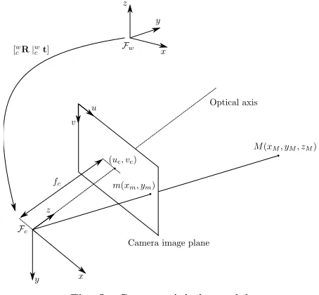
In this work, an image point is considered as a visual feature. To model a visual servoing system, the projection of an object with respect to the pinhole camera system must be described. Figure 5 illlustrates the camera pinhole model. In Figure 5, the coordinates vector of a 3D point
M= [xM, yM, zM]T is projected in 2D camera image plane
coordinates as m = [xm, ym]T. Note that the image point coordinates vector m is used as the image features vector s. The projection from 3D into 2D coordinates is described as
xm= xM
zM = u−uc
fcku (20)
ym= yM zM =
v−vc
fckv (21)
Fig. 5: Camera pinhole model
where (u, v) are the coordinates of the projected point m expressed in pixels, (uc, vc) are the image plane principal coordinates and fc is the camera lens focal length,ku is the pixel size in the udirection andkv is the pixel size in the v direction. Lets first, consider the transformation of(xM, yM)
into(xm, ym). The first derivative of (20) and (21) are derived as
˙
xm= xM˙ zM−xMzM˙ (zM)2
(22)
˙
ym= y˙MzM−yMz˙M
(zM)2 (23)
The mapping of the camera velocity into the velocity of a 3D point can be described using a well-known formula as follows
˙
M= −vc−[ωc]×M (24)
where the skew symmetric matrix of[ωc]× is computed as
[ωc]×=
0 −ωz ωy
ωz 0 −ωx
−ωy ωx 0
(25)
Thus we have
˙
xM = −x˙c−ωyzM+ωzyM
˙
yM = −yc˙ −ωzxM+ωxzM (26)
˙
zM = −zc˙ −ωxyM+ωyxM
Substituting (26) into (22) and (23), the velocity of the projected point on the image plane associated with the cam-era movement described in (19) can be formulated where
˙
s= [ ˙xm,ym˙ ]Tand the interaction matrixL∈ R2×6is derived
as
L=
− 1
zM 0
xm
zM xmym −(1 +x
2
m) ym
0 − 1 zM
ym
zM (1 +y
2
m) −xmym −xm
(27)
the minimum number of 3 points is required. Let’s denote a vector of 3 points ass= [s1,s2,s3]T, a new interaction matrix
can be obtained by stacking each individual interaction matrix of s1,s2 ands3, thereforeL= [L1,L2,L3]T∈ R6×6.
C. IBVS Control Law
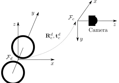
Let’s assume that the camera frame Fc and the robot local frame Fd is coincide, therefore it can be deduced that the camera velocity ξ˙c= ˙ξd. Substituting (17) into (19) yields
˙
s= LJω (28)
thus
ω= J†L†s˙ (29)
whereJ† andL† are generalised inverse of the robot Jacobian and the interaction matrix, respectively. Practically, the desired image features vector is constant, for instance the centre coordinates of the desired image features are on the centre of the camera image view. Therefore, in a simple form, the first derivative of (18) is expressed ase˙ = ˙s. The IBVS control law is designed to exponentially decrease the error e, thus it can be formulated thate˙ =−λewhereλis a positive constant describing how fast the error is regulated to zero. In the case where the camera frame is coincide with the robot frame, the IBVS control algorithm is computed as follows
ω= −λJ†L†e (30)
In most common case, the camera frame is not coincide with the robot frame. Thus, there is a transformation between the camera frame and the robot frame which denoted by its translation vector td
c and rotation matrix Rdc as shown in Figure 6.
Fig. 6: Transformation between camera frame and robot frame To relate the 3D velocity vector between coordinate frame, the velocity twist matrix is introduced into control law com-putation (30) as follows
ω= −λJ†[Vc d]−
1L†e (31)
where the velocity twist of the robot frame with respect to the camera frame Vc
d∈ R
6×6is computed by Vcd=
Rc
d [tcd]×Rcd
0∈ R3×3 Rc
d
(32)
and the skew symmetric matrix of the robot frame origin position with respect to camera frame (tc
d = [tx, ty, tz]T) is expressed as
[dcd]×=
0 −tz ty
tz 0 −tx
−ty tx 0
(33)
Using basic transformation formula between coordinate sys-tems, the relation of the homogeneous transformation matrix components between the camera frame and the robot frame can be obtained by
Rcd= [Rdc]T (34)
tcd= −[Rd
c]Ttdc (35) Indeed, the computation of the IBVS control law in (30) and (31) require the exact measurement of the robot physical model parameters such as: robot wheel diameterrwandL. In practice, due to the mechanical imprecission design, it is more ellegant to denotebJinstead ofJfor representing the estimated
robot Jacobian. It is also noted that the interaction matrixLin (27) is the function of the exact 3D and 2D parameters of the target object:ZM,xm andym. Those parameters, in fact can only be estimated considering the camera intrinsic parameters (e.g fc) and extrinsic parameters (Rc
d andt c
d) difficult to be obtained precisely during callibration process. Furthermore, a complex algorithm of pose estimation should be used in order to compute the estimated interaction matrix denoted as
b
L in every iteration of visual servoing process. Thanks to Chaumette and Hutchinson [5] for the detail discussion of the interaction matrix option where the desired target parameters are used. In this option, the computation of the interaction matrix is simpler where the computation of a complex pose estimation algorithm is not required while the exponential decreasing error can still be achieved. Moreover, the estimated interaction matrixLbbecomes constant, it is not necessary that b
L has to be computed in every iteration. In this work, the estimated robot Jacobian and interaction matrix of the desired target were used, therefore, the expression of the IBVS control law is described as
ω= −λbJ†Lb†e (36)
or
ω= −λbJ†[Vbdc]−1Lb†e (37)
if the camera frame is not coincide with the robot frame. III. STABILITYANALYSIS
The stability of the proposed closed-loop system (36) or (37) can be verified in terms of Lyapunov stability. Lets define the quadratic Lyapunov candidate function as
V =eTe (38)
Thus, the time derivative of the quadratic Lyapunov candidate function (38) can be computed as
˙
Lets denote (LJ) as A, (J†L†) as A†. The estimated of those two matrices denoted as Ab andAb†, respectively. Using
˙
e= ˙s and equation (29), the time derivative of the quadratic Lyapunov candidate function (39) can be expanded as
˙
V = −λeTAω (40)
In fact, the angular velocity vectorωwas computed using the estimated robot jacobian and the estimated interaction matrix, therefore V˙ can be obtained by
˙
V = −λeTAAb†e (41)
˙
V = −λeTA(Ab†+A†−A†)e (42)
˙
V = −λeTAA†e−λeTAe (43) whereis the error between the estimated and the actual of the inverse robot Jacobian and the interaction matrix,Ab† andA†,
respectively. The system asymptotic stability can be achieved if condition below is ensured:
kAA†k = kIk>kAk (44) Indeed, if the estimated robot Jacobian and the interaction matrices are equal to the actual values,=0then the system asymptotic stability is guaranteed,V˙ ≤0.
IV. IBVS ROBUSTNESSDUE TOCAMERACALLIBRATION ERROR
It is also necessary to prove that the IBVS control law is a robust system due to the camera callibration error. Firtly, lets recall the fundamental 3D-2D mapping from a pin-hole camera model which described as follows:
u v
1
=
fcku 0 uc
0 fckv vc
0 0 1
xm ym
1
(45)
xi = Wxm (46)
By considering that the intrinsic camera parameter matrix
c
W is used and the fact that the IBVS uses direct image measurement on the image space as the contoller input, it can be deduced that
b
xm = Wc−1xi (47)
Substituting (46) into (47)
b
xm = Wc−1Wxm (48)
where
c
W−1W =
fcku
b
fcbku
0 uc−buc b
fcbku
0 fckv
b
fcbkv
vc−bvc
b
fcbku
0 0 1
(49)
=
b
Ku 0 Ub
0 Kbv Vb
0 0 1
(50)
Note thatfc,kuandkvare always positive. The first derivative of (48) can be formulated as
˙
b
xm = Kub xm˙ (51)
˙
b
ym = Kbvy˙m (52)
Thus in compact form, it can be deduced that
b
L = KLb (53)
where
b
K =
"
b
Ku 0
0 Kvb #
>0 (54)
Lets consider thatJ≈Jbthen the first derivative of the defined
Lyapunov function can be expressed as
˙
V = −λeTLLb†e (55)
= −λeTLL†Kb−1e≤0 (56)
thus the asymptotic stability of the system can be ensured. Indeed, if the kinematic robot Jacobian formulation is too far from the actual then the system can be unstable.
V. EXPERIMENTALRESULTS A. Experimental Setup
where the subscript 1 to 4 indicate the index of each dot. To simplify the notation for the detail explanation in the next discussion, s = [s1, s2, s3, s4, s5, s6, s7, s8] is used instead.
Thanks to ViSP libraries that provides functions to extract and track the dot image on the image view of the camera. A simple self-explanatory diagram block of the experimental setup is shown in Figure 8.
Fig. 8: Diagram block of the experimental setup
B. Simulation
Robot Cont rol Variables
T
ra
ns
ta
ti
ona
l
and
R
ot
at
io
na
l
Ve
lo
ci
ti
es
-0.6 -0.4 -0.2 0 0.2 0.4 0.6 0.8 1
Time (s)
0 0.5 1 1.5 2 2.5
v ω
Fig. 9: Robot velocities
Robot Trajectory
y(
me
te
rs
)
-0.25 -0.2 -0.15 -0.1 -0.05 0 0.05
x(meters)
0 0.2 0.4 0.6 0.8 1 1.2
pr
Fig. 10: Robot trajectory
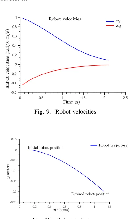
A simulation test was conducted to complement the system analysis. The simulation analysis used the robot velocities, the robot trajectory, the image feature error, the norm of the image feature error and the robot wheel angular velocities
Image Features Error e
e,
me
te
rs
-0.1 -0.05 0 0.05 0.1 0.15 0.2 0.25 0.3 0.35
Time (s)
0 0.5 1 1.5 2 2.5
e1 e2 e3 e4 e5 e6 e7 e8
Fig. 11: Image feature error
Fig. 12: Image feature error at initial robot pose
Fig. 13: Image feature error at desired robot pose
Error Trajectory
e
0 0.05 0.1 0.15 0.2 0.25 0.3
Time (s)
0 0.5 1 1.5 2 2.5
||e||
Fig. 14: Norm of the image feature error
Robot Wheel Velocit ies
Ome
ga
(
ω
)
0 5 10 15 20 25 30
Time (s)
0 0.5 1 1.5 2 2.5
ωR
ωl
Fig. 15: Robot wheel angular velocities
from pixels to meters were done using a simple pinhole camera model. Within the camera image view, the four dots image at the initial robot pose and the desired robot pose were captured as shown in Figure 12 and Figure 13, respectively. The trajectory of the norm of the image feature error is plotted in Figure 14. The error norm trajectory decreased exponentially as expected. Finally, the smooth convergence of the output of the MBVS control method, ω, was achieved as shown in Figure 15.
C. Realtime
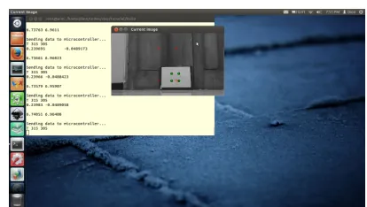
Fig. 16: A captured ubuntu terminal of the Beaglebone Black Realtime experiments were conducted succesfully. In this section, some images were captured from one of the
exper-Fig. 17: Bird views of the captured robot motion
Fig. 18: Captured image feature during the robot motion
iments to illustrate the performance of the MBVS method. Figure 16 shows the captured ubuntu terminal run on the Beaglebone Black during the robot motion. It is shown that the terminal printed the program messages to send the velocity command to the robot internal controller through UART communication port.
VI. CONCLUSION
An IBVS control strategy for a differential drive mobile robot navigation using single camera has been discussed in this paper. The detail fundamental development of the method has been presented. The stability and the system robustness in the presence of the camera callibration error have been discussed in detail. The perfomance analysis has been carried out in both simulation and realtime experiments using a differential drive robot prototype. The coordinates of the four dots image were used as the image features. The trajectory of the image features vector and its errors, the robot pose trajectory, and also the robot velocities have been shown to show the performance of the MBVS system. It has been shown that the norm of the image feature error vector decreased exponentially. In realtime experiments, photos have been taken to show the setup and also the motion of the robot from the initial position to the desired position.
ACKNOWLEDGMENTS
The authors would like to thank to the Indonesian Direc-torate General of the Higher Education (DIKTI) and Malang State Polytechnic who have supported this research project.
REFERENCES
[1] H. Rashid and A. K. Turuk, “Dead reckoning localization technique for mobile wireless sensor networks.”CoRR, vol. abs/1504.06797, 2015. [2] H. Bao and W.-C. Wong, “A novel map-based dead-reckoning algorithm
for indoor localization.” vol. 3, no. 1, pp. 44–63, 2014.
[3] A. Rudolph, “Quantification and estimation of differential odometry errors in mobile robotics with redundant sensor information.” I. J.
Robotic Res., vol. 22, no. 2, pp. 117–128, 2003.
[4] H. M. Becerra and C. Sags, “Pose-estimation-based visual servoing for differential-drive robots using the 1d trifocal tensor.” inIROS. IEEE, 2009, pp. 5942–5947.
[5] F. Chaumette and S. Hutchinson, “Visual servo control. i. basic ap-proaches,”Robotics Automation Magazine, IEEE, vol. 13, no. 4, pp. 82–90, Dec 2006.
[6] ——, “Visual servo control. ii. advanced approaches [tutorial],”Robotics
Automation Magazine, IEEE, vol. 14, no. 1, pp. 109–118, March 2007.
[7] I. Siradjuddin, T. McGinnity, S. Coleman, and L. Behera, “A com-putationally efficient approach for jacobian approximation of image based visual servoing for joint limit avoidance,” inMechatronics and
Automation (ICMA), 2011 International Conference on, Aug 2011, pp.
1362–1367.
[8] I. Siradjuddin, L. Behera, T. McGinnity, and S. Coleman, “Image-based visual servoing of a 7-dof robot manipulator using an adaptive distributed fuzzy pd controller,”Mechatronics, IEEE/ASME Transactions on, vol. 19, no. 2, pp. 512–523, April 2014.
[9] ——, “A position based visual tracking system for a 7 dof robot manipulator using a kinect camera,” inNeural Networks (IJCNN), The
2012 International Joint Conference on, June 2012, pp. 1–7.
[10] F. Janabi-Sharifi, L. Deng, and W. J. Wilson, “Comparison of basic visual servoing methods,”Mechatronics, IEEE/ASME Transactions on, vol. 16, no. 5, pp. 967–983, Oct 2011.
[11] P. Cigliano, V. Lippiello, F. Ruggiero, and B. Siciliano, “Robotic ball catching with an eye-in-hand single-camera system,”Control Systems
Technology, IEEE Transactions on, vol. 23, no. 5, pp. 1657–1671, Sept
2015.
[12] V. Lippiello, B. Siciliano, and L. Villani, “Position-based visual servoing in industrial multirobot cells using a hybrid camera configuration,”
Robotics, IEEE Transactions on, vol. 23, no. 1, pp. 73–86, Feb 2007.
[13] D. Jung, J. Heinzmann, and A. Zelinsky, “Range and pose estimation for visual servoing of a mobile robot.” inICRA. IEEE Computer Society, 1998, pp. 1226–1231.
[14] A. Cherubini, F. Chaumette, and G. Oriolo, “A position-based visual servoing scheme for following paths with nonholonomic mobile robots.” inIROS. IEEE, 2008, pp. 1648–1654.
[15] P. Rives, F. Chaumette, and B. Espiau, “Visual servoing based on a task function approach,” inExperimental Robotics I, ser. Lecture Notes in Control and Information Sciences, V. Hayward and O. Khatib, Eds. Springer Berlin Heidelberg, 1990, vol. 139, pp. 412–428. [Online]. Available: http://dx.doi.org/10.1007/BFb0042532
[16] E. Marchand, F. Spindler, and F. Chaumette, “Visp for visual servoing: a generic software platform with a wide class of robot control skills,”
IEEE Robotics and Automation Magazine, vol. 12, no. 4, pp. 40–52,
December 2005.