Abstract— Game theory is the formal study of decision-making where several players must make choices that potentially affect the interests of the other players. In this paper, we develop a combined computer oriented technique for solving game problems. In this technique, we implement Minimax-Maximin method, rectangular game, and convert the resulting game into Linear Programming (LP) problem. Finally, to find out the strategies of both players, we incorporate the usual Simplex method of Dantzig [11]. We develop our computer technique by using the programming language MATHEMATICA [16]. We will show the efficiency of our program for saving labor and time for solving game problems by presenting a number of numerical examples.
Index Term— Game, Linear Programming, Minimax-Maximin, Simplex, Strategy.
I. INTRODUCTION
Game theory is a mathematical theory that deals with the general features of competitive situations like parlor games, military battles, political campaigns, advertising and marketing campaigns by competing business firms and so forth. It is a distinct and interdisciplinary approach to the study of human behavior. The disciplines most involved in game theory are mathematics, economics and the other social and behavioral sciences. Game theory (like computational theory and so many other contributions) was founded by the great mathematician John von Neumann [23]. The concepts of game theory provide a language to formulate structure, analyze, and understand strategic scenarios. Game theory bears a strong relationship to LP, since every finite two person zero sum game can be expressed as a LP and conversely every LP can be expressed as a game. If the problem has no saddle point, dominance is unsuccessful to reduce the game and the method of matrices also fails, then LP offers the best method of solution. So far several authors namely Bansal [2], Martin [3], Stephen [1], Thedor [4] and many other authors proposed different types of theoretical discussion of game problems with their strategies also. But they didn‟t discuss computational procedure of game theory. Also none of them discussed the whole problem comprehensively. For this, there is a need to develop a technique which can address all type of game problems within a single framework. In this paper, we develop such a computer technique to find their strategies and the value of the game.
Haridas kumar Das is with the Department of Mathematics, University of Dhaka, Dhaka, Bangladesh.
(Mobile: +88-01557191305, e-mail:[email protected]) M Babul Hasan is with the Department of Mathematics, University of Dhaka,
Dhaka, Bangladesh.
(Mobile:+88-01720809792, e-mail:[email protected]
The rest of the paper is organized as follows. In Section II, we will discuss about different definitions of LP and game theory with some relevant theorems and propositions. In Section III, we will give a short discussion of simplex method and Minimax-Maximin method for solving game problems. A short discussion of rectangular 2×2 game will be given in section IV. In Section V, we will present our prime object by showing the construction of the generalized m × n computer technique with some numerical examples for the justification of our program. Also time comparison in second is given in Section VI. An over view focus on the above sections will be viewed in Section VII.
II. PRELIMINARIES
In this section, we briefly discuss some definitions of L P and game theory. We also include some propositions and theorems. For this, we first briefly discuss the general L P problems.
Consider the standard L P problems as follows, Maximize Z= x (1) Subject to Ax (≤, =, ≥) b (2) x ≥ 0 (3)
Where A is an m × n matrix and x=(x1, x2, x3,…….. xn), b =(b1, b2,
b3,…….. bm)T are column vectors. We shall consider any number of
rows and columns, b≠0 and the system of linear equations are given in equation (2).We shall also denote the ith column of A by
A(i) .
A. Objective function
The linear function z = = c1x1 + c2x2 + … … … + cnxn which is to be maximized (or minimized) is called objective function of the general linear programming problem (GLPP).
B. Constraints
The set of equations or inequalities is called the constraints of the general linear programming problem. Ax (≤, =, ≥) bis the set of constraints in the GLPP.
C. Solution of GLPP
An n-tuple (x1, x2, … … , xn) of real numbers which satisfies the constrains of a GLPP is called the solution of GLPP.
D. Feasible Solution
Any solution to a GLPP which also satisfies the nonnegative restrictions of the problem is called a feasible solution to the GLPP [8]. Or, A feasible solution to the LP problem is a vector x
An Algorithm and Its Computer Technique for
Solving Game Problems Using LP method
112303-8585 IJBAS-IJENS © June 2011 IJENS
= (x1, x2, … … , xn) which satisfies the conditions
i, i = 1, … … , m and j = 1, … … , n; xi ≥ 0.
E. Matrix Form
Suppose we have found the optimal solution to (1). Let BVi be the basic variable for row i of the optimal tableau. Also define BV = {BV1, BV2, … … , BVm} to be the set of basic variables in the optimal tableau, and define the m × 1 vector as,
xBV =
We also define NBV = the set of nonbasic variables in the optimal tableau
xNBV = (n - m) × 1 vector listing the nonbasic variables (in any desired order)
Using our knowledge of matrix algebra, we can express the optimal tableau n terms of BV and the original LP (1). Recall that
c1, c2, … … cn are the objective function coefficients for the variables x1, x2, . . . , xn (some of these may be slack, excess or artificial variables).
Here, cBV is the 1 × m row vector .
Thus the elements of cBV are the objective function coefficients for the optimal tableau‟s basic variables. cNBV is the 1 × (n - m) row vector whose elements are the coefficients of the no basic variables (in the order of NBV). The m × m matrix B is the matrix whose jth column is the column for BVj in (1). aj is the column (in the constraints) for the variable xj in (1). N is the m × (n - m) matrix whose columns are the columns for the non-basic variables (in the NBV order) in (1). The m × 1 column vector b is the right-hand side of the constraints in (1).
F. Game
A game is a formal description of a strategic situation [25].
G. Strategy
A strategy of a player „p‟ is a complete enumeration of all the actions that he will take for every contingency that might arise [20].
H. Pay-off
The pay-off is a connecting link between the sets of strategies open to all the players. Suppose that at the end of a play of a game, a player pi (i=1,2,……….,n) is expected to obtain an
amount vi, called the pay-off to the player pi. .
I. Pay-off matrix
A pay-off matrix is the table that represents the pay-off from player II to player I for all possible actions by players [22].
J. Fair game
A game is said to be fair game if the value of the game is zero.
K. Pure strategy
A pure strategy for player I (or player II) is the decision to play the same row (or column) on every move of the game [20]. Consider the matrix game A= for two players. If both players employ pure strategies, the outcome of each move is exactly the same and the game is completely predictable. For example, if player I always chooses the ith row and player II always chooses the jth column, then on every play of the game player I receive units from player II.
L. Mixed strategy
A mixed strategy is an active randomization, with given probabilities that determine the player‟s decision. As a special case, a mixed strategy can be the deterministic choice of one of the given pure strategies.
Suppose player I does not want to play each row on each play of the game with probability 1 or 0, as was the case with pure
strategies. Instead, suppose he decides to play row i with probability xi with i=1,2,…..,m, where more than one xi is greater
than zero, and I = 1.This decision is denoted by
X=
is called a mixed strategy for player I [18]. In like manner, if player II decides to play column j with probability yj with
j=1,2,……,n where more than one yi is greater than zero, and
I =1.
Then
Y=
M. Player
A player is an agent who makes decisions in a game.
N. Strategic form
A game in strategic form, also called normal form, is a compact representation of a game in which players simultaneously choose their strategies. The resulting payoffs are presented in a table with a cell for each strategy combination.
O. Two-person zero-sum game
A game is said to be zero-sum if for any outcome, the sum of the payoffs to all players iszero. In a two-player zero-sum game, one player‟s gain is the other player‟s loss, so their interests are diametrically opposed [21].
P. Saddle point
called the value of the game and is obviously equal to the maximin and minimax values of the game.
Theorem 2.1
If mixed strategies are allowed, the pair of mixed strategies that is optimal according to the minimax criterion proves a stable solution with V= = , so that neither player can do better by unilaterally changing her or his strategy [10, 26].
Theorem 2.2
In a finite matrix game, the set of optimal strategies for each player is convex and closed [14].
Theorem 2.3
Let, v be the value of an m × n matrix game. Then if
Y= is an optimal strategy
for player II with > 0, every optimal strategy x for player I must have the property
Similarly, if the optimal strategy x has > 0, then the optimal strategy y must be that
Proposition 2.1: The set S= {x | Ax = b, x ≥ 0 } is convex.
Proposition 2.2:x ≥ 0 is a basic nonnegative solution of (2) if and
only if x is a vertex of (1).
Proposition 2.3:If the system of equations (2) has a nonnegative solution, then it has a basic nonnegative solution.
Proposition 2.4:S has only a finite number of vertices [15, 17].
III. TWO EXISTING METHODS [13,15]
In this section, we briefly discuss of the usual Simplex method and Minimax-Maximin method.
3.1. Simplex Method
The Simplex method is an iterative procedure for solving linear programming problems expressed in standard form. In addition to the standard form, the Simplex method requires that the constraint equations be expressed as an economical system from which a basic feasible solution can be readily obtained. If the standard faint of LP is not in canonical form, one has to reduce it to a variable. Then we remove these artificial variables by applying two- phase method or Big-M method. The Simplex method is developed by George B. Dantzig [11] in 1947. The Simplex method has a wide range of applications including agriculture, industry, transportation and other problems in economics and management science.
3.2. Minimax-Maximin pure strategies
Since each player knows that the other rational and same objective that is, to maximize the pay offfrom the other player, each might
decide to us the conservative minimax criterion to select an action. That is, player I examines each row in the payoff matrix and selects the minimum element in each row, say pij with i=1,2
………,m. Then he selects the maximum of these minimum elements, say prs.
Mathematically, V=prs=max[min(pij)]
The element prs is called the maximin value of the game, and the
decision to play row r is called the maximin pure strategy. Likewise, player II examines each column in the payoff matrix to the column with the smallest maximum loss.Let,
V=ptu=min[max(pij)]
Then ptu is called the minimax value of the game and the decision
to play column u is called minimax pure strategy. It can be shown that, the minimax value v represents a lower bound on a quantity called the value of the game, and also v represents a upper bound on the value of the game.
IV. RECTANGULAR 2×2GAME
In this section, we present a short discussion about 2×2 particular game problems [19].
First, consider a 2×2 game with the payoff matrix.
Let xi be the probability player II plays row I with i =1, 2, and let
yj be the probability player I plays column j with j=1, 2. Since
Player II
Player I … … … … … (4.a)
I =1 and I =1
So we can write, x2=1- x1 and y2= 1 - y1.
The saddle point is necessarily the value of the game. If a saddle point does not exist, then we have to follow the following procedure. Let,
The optimal strategy of player I is =
The optimal strategy of player II is =
y*1= … … … … (4.b)
y*2=1-y*1 … … … … (4.c)
x*1= … … … … (4.d)
x*2=1-x*1 … … … (4.e)
These will be optimal minimax strategies for player I and player II respectively.
Finally the value of the game is
112303-8585 IJBAS-IJENS © June 2011 IJENS
(1-y*1)(1-x*2 ) … … … … … …(4.f)
V. SOLVING GAME PROBLEMS REDUCING INTO L P
In this section, we discuss generalized m × n game problems for converting it into LP to find the two players strategies with the help of LP method.
In many applications, one needs to compute basic solutions of a system of linear equations. For example, in dealing with many linear programming problems, especially degenerate and cycling problems [5], it is often more convenient to locate the extreme points by applying the usual simplex method. In this paper, we outline a procedure for finding two strategies of a system of m equations in n variables and develop a computer procedure using the computer algebra MATHMATICA [11, 16]. For this, we first apply Minimax-Maximin and Rectangular method to find game value in section 5.2.1. Finally, we will solve [5.a] by usual Simplex method in our code in section 5.3.1. On the other hand, our method yields the game value easily.
5.1 A Short Discussion of m × n Game [10]
Any Game with mixed strategies can be solved by transforming the problem to a linear programming problem.Let, the value of game is v. Initially, player I acts as maximize and player II acts as minimize.But after transforming some steps when we convert the LP then inverse the value of the game.For this objective function also changes.
First consider, the optimal mixed strategy for player II,
Expected payoff for player II = ijyjxi and the player II
strategy (x1, x2, ... , xm) is optimal if ijyjxi ≤ v for all
opposing strategies i.e. player I is (y1,y2,...,yn).After some
necessary calculations we get the followng two forms of player II and player I respectively.
Player II :
Maximize, = x1+x2+………. .+xm
Subject to,
p11x1 +p12x2 +……….+p1nxn ≤ 1
p21x1 +p22x2 +……….+p2nxn ≤ 1
….……… … … 5(a)
pm1x1 +pm2x2 +……….+pmnxn ≤ 1
x1 + x2 + ………+xn =1
and xj 0 ,for j=1 , 2, ………n.
Player I:
Minimize, = y1+y2+……….……..+ym
Subject to,
p11y1 +p21 y2 +………...….+pm1ym ≥ 1
p12y1 +p22y2 +……….+pm2ym ≥ 1
………. … … (5.b)
P1ny1 +p2ny2 +……….+pmnym ≥ 1
y1 + y2 + ………...……+ym =1
and y
i0 ,for i=1 , 2, …………..…m.
.We can solve (5.a) and (5.b) by suitable L P method such as usual simplex method or Big M simplex method or Primal-dual simplex method [7]. In this paper we will develop a computer technique incorporate with usual Simplex method.
5.1.1 Numerical Example
All game problems can be solved by our procedure. Here we consider a real life problem, which illustrates the implementation and advantage of the above procedure.
Two oil companies, Bangladesh Oil Co. and Caltex, operating in a city, are trying to increase their market at the expense of the other. The Bangladesh (B. D.) Oil Co. is considering possibilities of decreasing price, giving free soft drinks on Rs. 40 purchases of oil or giving away a drinking glass with each 40 litter purchase. Obviously, Caltex cannot ignore this and comes out with its own program to increase its share in the market. The payoff matrix forms the viewpoints of increasing or decreasing market shares is given in table below.
Caltex
B.D
Oil Co.
Decrease price
Free soft drinks on Rs.40 purchase
Free drinking glass on 40 liters or so
Decrease price
4% 1% -3%
Free soft drinks on Rs.40 purchase
3 1 6
Free drinking glass on 40 liters or so
-3 4 -2
Determine the optimum strategies for the oil company [12].
5.1.2 Solution
The Solution can be found step by step in [12].
Best strategies for A (B. D. Oil Co.) = (1/4, 1/2, 1/4).Best strategies for B (Caltex) = (27/92, 62/92, 3/92).Value of the game (for A) =7/4.
5.2 Algorithm
In this section, we first discuss the algorithm of the game by Minimax-Maximin,2×2 strategies and for the modified matrix of the game problems.
Sub step (I): Search the maximum element from each row of the payoff matrix of equation (4.a).
Sub step (II): Search the minimum element from each column of the payoff matrix of equation (4.a).
Sub step (III): If they coincide then the value of the game is V= Maximin element=Minimax element. Then Stop .If we fail to get such value, go to Sub step (IV).
Sub step (IV): Find the mixed strategies for player I using (4.b) and (4.c).
Sub step (V): Find the mixed strategies for player II using (4.d) and (4.e).
Sub step (VI): Finally, we get value of the game by (4.f). Otherwise go to Step (2) for m , n >2.
Step (2): Search the minimum element from each row of the reduced payoff matrix and then find the maximum element of these minimum elements.
Step (3): Search the maximum element from each column of the reduced payoff matrix and then find the minimum element of these maximum elements
.Step (4): For the player Iif the Maximin less than zero then find k which is equal to addition of one and absolute value of Maximin.
Step (5): For the player IIif the Minimax less than zero then find k which is equal to addition of one and absolute value of Minimax.
Step (6): If Maximin and Minimax both are greater than zero then k≥0.
Step (7): Finally to get the modified payoff matrix adding k with each payoff elements of the given payoff matrix.
Step (8): Then to find the mixed strategies with game value of the two players, follow the algorithm of section 5.3.
5.2.1 Program
In this section, we construct a computer technique for finding the modified matrix. Also we use Minimax-Maximin for finding value of the game and Rectangular 2×2 game also find value of the game with their strategiesusing MATHEMATICA [11, 16 ] .
5.2.1.1 Input of Example 5.1.1
5.2.1.2 Output of Example 5.1.1
5.3 Algorithm for player I and player II
In this section, we present our computational procedure incorporated with simplex method in terms of some steps for finding their strategies with the game value from the modified matrix for m × n game problems.
112303-8585 IJBAS-IJENS © June 2011 IJENS
Step (2): We will get equations (5.a) and (5.b)for the player IIand player I respectively.
Step (3): We take input for player II from the equation (5.a). Step (4): Define the types of constraints. If all are of “≤” type goes to step (6).
Step (5): We follow the following sub-step.
Sub-step (I): Express the problem in standard form.
Sub-step (II): Start with an initial basic feasible solution in canonical form and set up the initial table.
Sub-step (III): Use the inner product rule to find the relativeprofit factors
̅
as follows̅
̅
-
(inner product of and the column corresponding to in the canonical system).Sub-step (IV): If all
̅
, the current basic feasible solution is optimal and stop. Otherwise select the non-basic variable with most positive̅
to enter the basis.
Sub-step (V): Choose the pivot operation to get the table and basic feasible solution.
Sub-step (VI): Go to Sub-step (III).
Step (6): At first express the problem in standard form by introducing slack and surplus variables. Then express the problem in canonical form by introducing artificial variables if necessary and form the initial basic feasible solution. Go to Sub-step (III).
Step (7): If any
̅
corresponding to non-basic variable is zero, the problem has alternative solution, take this column and go to Sub-step (V).Step (8): Finally, we find all the stratigies for player II is in corresponding their right hand side (RHS) and strategies of player I is in corresponding the
̅
of the slack variables.
Step (9): Calculate the value of the object functions for each feasible solution.
5.3.1 Program
112303-8585 IJBAS-IJENS © June 2011 IJENS
The program shown in the Section 5.3.1 with an algorithm in Section 5.3 is the general program for finding the strategies of m × n game problems.
To take input as in matrix form, we convert the modified matrix as a form of the equation (5.a) in section 5.1.
5.3.1.1 Input for the player II of Example 5.1.1
5.3.1.2 Output for the player I and player II of Example 5.1.1
Hence the output of both player strategies and the game value coincide with the given example 5.1.1.
Moreover, to justify our technique we present another numerical example in this section.
5.1.2 Numerical Example
The payoff matrix of a game is given below.
A B
I II III IV V VI
1 4 2 0 2 1 1
2 4 3 1 3 2 2
3 4 3 7 -5 1 2 4 4 3 4 -1 2 2 5 4 3 3 -2 2 2 Find the best strategy for each player, and the value of the game to A and B [12].
5.1.3 Solution
The Solution can be found step by step in [12]. The value of the game is 13/7.
5.1.2.1 Programming Input of Example 5.1.2 in section 5.2.1
5.1.2.2 Programming Output of 5.1.2 in Section 5.2.1
5.1.2.4 Programming Input of 5.3.1 for player I & II from section 5.1.2.2
5.1.2.4 Programming Output of 5.1.2 for player I & II in section 5.3.1
Therefore we get from the output from Section 5.1.2.4
Optimal strategy for player A is: (0, 6/7, 1/7, 0, 0) and
112303-8585 IJBAS-IJENS © June 2011 IJENS
Game value: =13/7.
Hence the output of two player strategies and the game value coincides with that of the given example in Section 5.1.2.
Using the combined program, we have to „Local Kernel Input‟ 5, 6, 0, 0 respectively as to indicate the number of rows, number of columns, number of greater than type constraints and the value of k from the modified matrix. Also no greater type constraints, „l‟ five time to indicate five less than type constraints and all other inputs as prompt requirement. The program showed the simplex table iteration by iteration. And the strategies obtained which is identical with that of the Simplex method.
To solve 3×3 or higher Games also, the first step is to look for a saddle point for, if there is one, and then Game is readily solved. If the Game is 2×2 it can easily solved by the methods described in section 4. If the pay-off matrix is 2×n (or m×2 or 3×3 size), it can be solve by algebraic method, method of matrices and iterative method. But for the higher dimensions it cannot be solved successfully by the prescribed methods. But our computer technique can be solved m × n Game problems easily by method of LP.
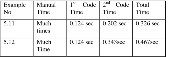
VI. TIMECOMPARISN
In this section, we compare the time required to solve the game problems by our method with that of the manual solution. Here, we use the command “TimeUsed[ ]” for calculating the required time in our code to find the output.
Example No
Manual Time
1st Code Time
2nd Code Time
Total Time
5.11 Much
times
0.124 sec 0.202 sec 0.326 sec
5.12 Much
Time
0.124 sec 0.343sec 0.467sec
Hence, we can say that our code is highly powerful for saving time.
VII. CONCLUSION
In this paper, we developed a combined computer technique for solving game problems. This computer technique incorporated Minimax-Maximin Method, Rectangular 2×2 Game and LP Method. Our technique can address any game problem within a single framework. We demonstrated our program and discussed the changes step by step throughout our paper. The program developed by us is a powerful computer technique. Hand calculation is very tough and time consuming for analyzing the game problems with large number of variables and constrains, where we can do the same problems by our program very easily. Nowadays, the world is being ruled by the fastest. So, we must try to finish our job as fast as we can. Finally, we can say that our computer oriented technique with MATHEMATICA for analyzing game problems is more efficient than any other methods.
VIII. ACKNOWLEDGEMENT
The author wishes to thank reviewers of IJBAS-IJENS for their important suggestions which helped to improve the presentation.
REFERENCES
[1] Stephen Wolfram, “Mathmatica”,Addision-wesley Publishing company,Menlo Park, California, Newyork(2000).
[2] S.Bansal,M.C.Puri, “A Min Max Problem”, Zeitschrift fur operations Research, Vol 24, 1980,Page 191-200.
[3] Martin J. Osborne, An introduction to game theory; Version: 2002/7/23.
[4] Theodore L.T. , Texas A&M University, Bernhard von Stengel, London School of Economics, “Game Theory”, CDAM Research Report LSE-CDAM-2001-09, October 8, 2001.
[5] E.M.L. Beale, “Cycling in the dual simplex algorithm”, Naval Research Logistics uarterly, Vol 2 (1955), No.4.
[6] Hasan M.B, Khodadad Khan A.F.M. and M. Ainul Islam(2001), “Basic solution of Linear Syestem of Equations through Computer Algebra”, “Ganit:j.Bangladesh Math”,Soc.21,pp.1-7. [7] Ravindran, Phillips and Solberg, “Operation Research Principles and
Practice ”.
[8] Saul I. Gauss,"Linear Programming Methods and Applications", Edition, Dover Publications, Inc, Mineola, New York [9] EDWARD L.KAPLAN, “Mathmatical Programming and
Games”,Printed in the United States of America.
[10] Gerald J. Lieberman, Frederick S. Hillier Stanford University, Frederick S. Hiller, Stanford University, “Introduction to Operation
Research”, edition, McGraw-Hill Book Co.
[11] G.B Dantzig, “Linear Programming and extension”,Princeton university press,Princeton,N,J(1962).
[12] P.K.Gupta,D.S Hira, "Problems IN Opereation Reasearch",S.Chand & Company LTD,Ram Nagar,New Delhi-110055.
[13] L.S.Srinath, Linear Programming Principlas and Applicatios, edition”,Affiliated east-west press PVT LTD.,New Delhi Madras Hyderabad(1975,1982).
[14] N.S.Kambo, “Mathmatical Programming Techniques,Revised edition”, Affiliated east-west press PVT LTD.,New Delhi Madras Hyderabad Banglore(1984,1991).
[15] Hamdhy.A.Taha, “Operation Research: An
introduction, edition”,Prentice Hall of India,PVT.LTD,New Delhi(1862).
[16] Eugene Don, “Theory and Problems of Mathmatica ”,Schaum’s Outline Series, McGRAW-HILL,New York San Francisco Washington,D.C.
[17] M. Marcus, ”A Survey of Finite Mathematics” . Houghton Mifflin Co. Boston.(1969).p(312-316).
[18] Thomas L. Saaty, “Mathematical Methods of Operations Research”,McGraw-Hill Book Company,Inc,New York St.Louis San Francisco .
[19] Stanley I. Grossman, “Applied Mathematics for the management, Life, and Social Sciences”,Wadsworth Publishing company,Belmont,California.
[20] M. Sasieni, A. Yaspan, L. Friendman, “Operations Research...methods and problems”, 9th edition,November, 1966,John Wiley & Sons,Int.
[21] Harvey M. Wagner, “Principles of Operations Research”,2th edition,Prentice-Hall of India Pv. Lt.,New Delhi-110001.
[22] McKinsey, J.C.C., “Introduction to the Theory of Games”, McGraw-Hill Book Company , Int., New York, 1952.
[23] Von Neumann, J., and O. Morgenstern, “Theory of Games and Economic Behavior”, second edition, Princeton University Press, Princeton, N.J., 1947.
[24] Williams, J.D., “The Compleat Strategyst”, McGraw-Hill Book Company, Int. , New York, 1954.
[25] Davis, M., “Game Theory: An Introduction”, Basic Books, New York, 1983.
[26] Meyerson, R. B., “Game Theory: Analysis of Conflict, Harvard University Press, Cambridge, MA, 1991
****
1 Haridas Kumar Das, Department of Mathematics, University of Dhaka, Dhaka-1000, Bangladesh, E-mail:[email protected].