(Research article)
An Approach for Cluster Analysis based upon Hierarchical Algorithm -
Agglomerative Algorithm
Neeraj Vermaa*, Pooja Grovera, Ajay Deepa
aDepartment of Computer Science & Engg., OITM, Hisar
Accepted 16 July 2012, Available online 1Sept 2012
Abstract
Cluster analysis is a method which is meant for classification of the data into natural groups. Recently Cluster analysis is linked with software automatic categorization system. A categorization system is one that is structured so that entities within the system with common features will be grouped together. This paper describes hierarchical algorithm – agglomerative algorithm for cluster analysis with empirical study.
Keywords: Cluster analysis, Hierarchical algorithm
1. Introduction
1
Software categorization defined as the activity of labeling software, belonging to different domains. Generally there are two different ways for making automatic classifiers. In a knowledge engineering approach, the knowledge of human experts is described as a set of rules, which are then used in the process of classification. The disadvantage of this approach is that it requires lot of effort to make human knowledge explicit and for each new domain a separate formulation of the rules need to done manually again. In a machine learning approach, the classifier is built automatically and classification for different domains can be learned using the same algorithm. The exactness of all automatic classification system is extremely reliant upon the effort and concern taken during process[1].A cluster analysis plays big role in software categorization. Cluster analysis is used to separate the data into bunch or groups where no prior information is available. It divides data into groups (clusters) that are meaningful, useful or both and then the clusters should be based on the original structure of the data. The cluster analysis is a vital tool in decision making and an effective method to obtaining solutions. The units within a cluster are as similar as possible, and clusters are also as different as possible. The main reasons for doing a cluster analysis are data exploration, visualization, data reduction, hypothesis generation. Partitioning or clustering techniques are used in many areas for a wide spectrum of problems. Cluster analysis
*Corresponding author's email: [email protected]
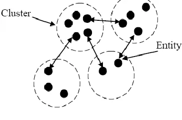
can be applied for graph theory, business area analysis, information architecture, information retrieval, resource allocation, image processing, software testing, galaxy studies, chip design, pattern recognition, economics, statistics and biology [2]. Figure-1 shows that the member entities of one cluster are not part of other clusters. The items which are to be clustered (the points) are represented by bullets. The dotted shapes signify clusters; the points within each dotted shape comprise a cluster. The goal of clustering methods is to extract an existing „natural‟ cluster structure. However, different methods may come up with different clustering. as a result, a particular algorithm may define a structure rather than find an existing one. It might even be the case that an algorithm „finds‟ a structure while there really is no natural structure in the data.
Figure-1
This paper includes four sections, Algorithmic approaches adopted for cluster analysis in section2; Euclidean Distance Metrics and Hierarchical Algorithms for cluster analysis presented in section 2.1 and section 2.2., lastly the conclusion is explained in section 3. International Journal of Engineering, Science and Metallurgy
2. Approach adopted
Cluster analysis is a well established field of research that has been applied to many different disciplines. Many research papers concluded that cluster analysis may also be fit for reengineering purposes and a number of different projects are currently pursuing this hypothesis. Cluster analysis discovers a natural structure within a set of entities. The method is based on discrete descriptions of these entities and is designed to deal with very complex relationships between these entities. Therefore cluster analysis is very well suited to software categorization which involves taking a group of functions with complex relationships involving data structures and other functions and merging them together in logically coherent groups.[3] There are a large number of techniques available, each of which may or may not be suitable for software categorization. Cluster analysis providing the relevant information about a characteristic can be extracted from the code. Firstly, we find out the similarity between two entities. Using the information in the data matrix and retrieved values and the similarity between the entities is calculated using the selected metric based on these values. There is a large number of similarity metrics designed for different purpose but Euclidean distance metric provides a more succinct overview.
The next step is concerned with the performance of the actual work of taking a dissimilar set of entities and grouping them into clusters. This work is carried out using a clustering algorithm. This paper focus on agglomerative hierarchical algorithms.
A. Distance Measure: An important component of a clustering algorithm is the distance measure between entity points. The tree clustering method calculates the dissimilarities (similarities) or distances between the different objects. Similarities are defined as a set of rules on that bases grouping or separation of items are done. This is a significant step to select a distance measure, which will calculate the similarities of two elements. This can be explained through the following figure.
Figure 1
Figure-2 shows distance between two closest entities. Notice that this is not only a graphic issue: the problem
arises from the mathematical formula, which is used to combine the distances between the single components of the data feature vectors into a unique distance measure. That can be used for clustering purposes as different formulas leads to different clustering.[4] And domain knowledge is used to direct the formulation of a suitable distance measure for each particular function. Data consisting of measures of dissimilarity between all pairs of two units can be represented using a dissimilarity matrix D of the form. The dissimilarity matrix D can be constructed by a distance measure, called a metric. The most commonly used distance measure is a Euclidean distance based on the sum of the squared differences between pairs of measurements
.
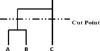
B. Hierarchical Algorithms: There are two kinds of hierarchical algorithms: agglomerative and divisive algorithms. The hierarchy of clusters is built in a manner that each level contains the same clusters, which are on the lower hierarchy. Following figure-3 shows an example of such hierarchy for three entities .
Figure-3
Figure-4
Figure-4 is graphically defining dendrogram for three entities. In divisive clustering all entities are contained in one cluster. In each step a cluster is split into two clusters. After N-1 steps there are N clusters each containing one entity?
Agglomerative hierarchical algorithms are most widely used technique as it is not feasible to judge all possible divisions of the first large clusters (2N-1-1 possibilities in the first step). Comprehensively, the algorithm consists of the subsequent steps:
• Compute the proximity matrix. • repeat
• Merge the closest two clusters.
• Update the proximity matrix to reveal the closeness between the new cluster and the original clusters. There are several regulations for deciding how the combined units should be treated. These rules are based on the idea linkage, the features of the two groups joined carried over to the combination of the groups.
Figure-5
Figure-5 Calculates the distance between various clusters. Suppose there are three clusters, A, B and C, with the distance between A and C being i and the distance between B and C being j. Let A and B are the most alike pair of entities, they must be clustered jointly into a new cluster, D. We then need to calculating the distance between C and D, K. The Three algorithms that have been used are differentiated by the way they deal with this issue.
• Single Linkage • Complete Linkage • Average Linkage
The single-linkage method, which is also called nearest-neighbor method.[6] The MIN version of hierarchical clustering, the closeness of two clusters is defined as the minimum of the distance (maximum of the similarity). Starting with all the points as single cluster and add links
between these points at a time, smallest links first, then these single links combines the points into clusters.
Figure-6
Figure 6 shows single link method for hierarchical clustering: K = min (i, j). The single link technique is fit for handling non-elliptical shapes, but is sensitive to noise and outliers. This form of linkage means that a single link is enough to join to groups, and this feature will allow clusters to elongate and not essentially sphere-shaped.
Figure-7
Figure-8
Figure 8 shows Group Average Link: K = (I, j) / 2. In the average linkage method, also called un-weighted pair-group method using arithmetic averages (UPGMA), the proximity of two clusters is defined as the average pair-wise proximity among all pairs of points in the different clusters. This is an intermediate approach between the single and complete link approaches. The average linkage method defines spherically-shaped clusters.
3. Empirical study
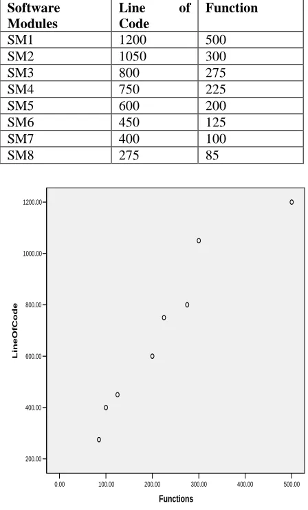
Consider a data set consisting of measurements of the variables Line of Code and Function for 8 Software Modules. The data set used is represented by the 8 x 2 data matrix.
Table- 1 Summary Table for Software Modules
Graph- 1
The dissimilarity matrix derived from the data matrix using Euclidean distance. Graph- 1 shows the graphical representation of eight modules.
Table- 2 Dissimilarity Matrix
Table- 2 shows the matrix of proximities between variables. These values represent the similarity or dissimilarity between each pair of items. For dissimilarities, larger values indicate items which are very different. Smaller values indicate items which are very similar. This relationship is reversed if a similarity measure is used.
Single Linkage Agglomeration Schedule: Table- 3
shows how the cases are clustered together at each stage of the cluster analysis. The clusters are formed by merging cases and clusters; and the process continues, until all cases are joined in one big cluster. At each stage, one case or cluster is joined with another case or cluster. For instance, in this example, cases 6 and 8 are joined at stage 3. This is shown in the Clusters Combined columns. When clusters or cases are joined, they are subsequently labeled with the smaller of the two cluster numbers. The Coefficients column (Table- 3) indicates the distance between the two clusters (or cases) joined at each stage. These values are based on the closeness among these clusters and linkage method is applied for this analysis. For a good cluster solution, a sudden jump in the distance coefficient (or a sudden drop in the similarity coefficient) is calculated. The stage before the sudden change indicates the optimal solution point for the merged clusters.
Table- 3 Single Linkage Agglomeration Schedule
500.00 400.00
300.00 200.00
100.00 0.00
Functions
1200.00
1000.00
800.00
600.00
400.00
200.00
Li
neO
fC
ode
Software Modules
Line of
Code
Function
SM1 1200 500
SM2 1050 300
SM3 800 275
SM4 750 225
SM5 600 200
SM6 450 125
SM7 400 100
The next part of the table shows the stage at which each cluster first appears. Single cases existed before we started the analysis, so they are indicated by zeroes here. In stage 5, cluster 3 is the cluster that was formed in stage 4 and cluster 3 is the cluster formed in stage 5.
Diagram- 1 Dendrogram A
The last column shows the subsequent stage at which the newly merged cluster is combined with yet another cluster. For example, the cluster formed in stage 4 next appears in stage 5, where it is merged with cluster 1. Diagram- 1 shows dendrogram, which is the two-dimensional representation of the tree. Generally, it is displayed with the largest cluster at the top and the smallest clusters at the bottom. The dendrogram is a graphical method, which is used to determine the number of clusters by looking at the heights. A specific clustering is attained by cutting the tree at some specific height. Large heights are suggested reasonably well separated clusters.
Table- 4 Complete Linkage Agglomeration Schedule
Conclusions
In this paper we have presented a general overview of the field of clustering. Clustering methods seem a very good starting point for the automatic categorization of modules. This is because the goal of clustering methods is to group related entities.
Diagram- 2 dendrogram B
An algorithm is selected which will satisfy the constraints of a good categorization of modules. The paper is also discussed in detail both Euclidean distance method for distance measure between two closest entities with the help of dissimilar matrix and agglomerative algorithm with the help of single and complete linkage method. Clustering technique plays an important role in data analysis and also extracts the most possible significant solution.
References
1. S. S. Parvinder, Madhu and S. Hardeep, “Automatic Categorzation of Software Modules” IJCSNS International Journal of Computer Science and Network Security,VOL.7 No.8, August 2007.
2. Popchev Ivan and Vania Peneva, “ Cluster – A Package for cluster analysis” 10th
annual international conference, 1988.
3. Wiggerts T.A., “Using Clustering Algorithms in Legacy Systems Remodularization” IEEE Fourth working conference on Reverse Engineering, pages 33-43, 06-08 oct. 1997.
4. Li Kai and Cui Lijuan, “Study of Models Clustering and Its Application to Ensemble Learning” Third International conference on Natural Computation (ICNC) 2007. 5. A. van Deursen and T. Kaupers, ”Identifying objects using
cluster and concept analysis” In Preceedings of the 21st International Conference on Software Engineering (ICSE 1999), Pages 246-255. IEEE Compter Society, 1999. 6. Y. Cheng, “Mean Shift, mode seeking, and clustering”
IEEE Transactions on Pattern Analysis and Machine Intelligence, Vol. 17, pp. 1197- 1203, 1999. 7. J. Handl and J. Knowles, “Exploiting the trade-
off-the benefits of multiple objectives in data clustering” In Proc. 3rd International Conference on Evolutionary Multi-Creiterion Optimization (EM‟O05), vol. 3410 of LNCS, pages 547-560, Springer-Verlag, 2005.