www.nat-hazards-earth-syst-sci.net/8/819/2008/ © Author(s) 2008. This work is distributed under the Creative Commons Attribution 3.0 License.
and Earth
System Sciences
A hydrometeorological model intercomparison as a tool to quantify
the forecast uncertainty in a medium size basin
A. Amengual1, T. Diomede2,3, C. Marsigli2, A. Mart´ın1, A. Morgillo2, R. Romero1, P. Papetti2, and S. Alonso1
1Grup de Meteorologia, Departament de F´ısica, Universitat de les Illes Balears, Palma de Mallorca, Spain 2ARPA-SIM Servizio IdroMeteorologico dell’Emilia-Romagna, Bologna, Italy
3Centro Interuniversitario di Ricerca in Monitoraggio Ambientale (CIMA), Universit`a degli studi di Genova e della Basilicata, Savona, Italy
Received: 4 December 2007 – Revised: 2 April 2008 – Accepted: 4 July 2008 – Published: 5 August 2008
Abstract. In the framework of AMPHORE, an INTERREG
III B EU project devoted to the hydrometeorological model-ing study of heavy precipitation episodes resultmodel-ing in flood events and the improvement of the operational hydrometeo-rological forecasts for the prediction and prevention of flood risks in the Western Mediterranean area, a hydrometeorolog-ical model intercomparison has been carried out, in order to estimate the uncertainties associated with the discharge pre-dictions. The analysis is performed for an intense precipita-tion event selected as a case study within the project, which affected northern Italy and caused a flood event in the upper Reno river basin, a medium size catchment in the Emilia-Romagna Region.
Two different hydrological models have been imple-mented over the basin: HEC-HMS and TOPKAPI which are driven in two ways. Firstly, stream-flow simulations ob-tained by using precipitation observations as input data are evaluated, in order to be aware of the performance of the two hydrological models. Secondly, the rainfall-runoff mod-els have been forced with rainfall forecast fields provided by mesoscale atmospheric model simulations in order to eval-uate the reliability of the discharge forecasts resulting by the one-way coupling. The quantitative precipitation fore-casts (QPFs) are provided by the numerical mesoscale mod-els COSMO and MM5.
Furthermore, different configurations of COSMO and MM5 have been adopted, trying to improve the description of the phenomena determining the precipitation amounts. In particular, the impacts of using different initial and boundary conditions, different mesoscale models and of increasing the horizontal model resolutions are investigated. The accuracy of QPFs is assessed in a threefold procedure. First, these
Correspondence to: A. Amengual
are checked against the observed spatial rainfall accumula-tions over northern Italy. Second, the spatial and temporal simulated distributions are also examined over the catchment of interest. And finally, the discharge simulations resulting from the one-way coupling with HEC-HMS and TOPKAPI are evaluated against the rain-gauge driven simulated flows, thus employing the hydrological models as a validation tool. The different scenarios of the simulated river flows – pro-vided by an independent implementation of the two hydro-logical models each one forced with both COSMO and MM5 – enable a quantification of the uncertainties of the precipita-tion outputs, and therefore, of the discharge simulaprecipita-tions.
Results permit to highlight some hydrological and me-teorological modeling factors which could help to enhance the hydrometeorological modeling of such hazardous events. Main conclusions are: (1) deficiencies in precipitation fore-casts have a major impact on flood forefore-casts; (2) large-scale shift errors in precipitation patterns are not improved by only enhancing the mesoscale model resolution; and (3) weak dif-ferences in flood forecasting performance are found by using either a distributed continuous or a semi-distributed event-based hydrological model for this catchment.
1 Introduction
820 A. Amengual et al.: Hydrometeorological simulations and forecast uncertainty A. Buzzi, M. C. Llasat, C. Obled, and R. Romero, 2005). The
Regional Hydrometeorological Service of Emilia-Romagna ARPA-SIM (Italy) and the Group of Meteorology of the Uni-versity of the Balearic Islands (Spain) are two of the associ-ated partners to this project. Within the AMPHORE frame-work, a set of hydrometeorological model simulations has been performed in order to improve the description of the phenomena determining the high precipitation amounts and to estimate the uncertainties associated with the hydrometeo-rological chain predictions. At this aim, this work focuses on one of the case studies selected in the project, an intense pre-cipitation episode which affected northern Italy and caused a flood event over the upper Reno river basin, a medium-sized catchment in the Emilia-Romagna Region.
One of the more important challenges for numerical weather modeling is to improve the quantitative precipita-tion forecasts (QPFs) for hydrological purposes. Concretely, the reliability and practical use of the flood forecasting sys-tem for the upper Reno river basin is strongly connected with the accuracy of QPFs provided by numerical weather pre-diction (NWP) models. These are useful to extend the de-sired forecast lead time beyond the concentration time of the basin. In fact, for the upper Reno river basin, rainfall obser-vations are not appropriate to drive the hydrological models, since they do not allow for the timely predictions required to implement an adequate emergency planning. The use of QPFs provided by NWP models is, therefore, fundamental. In general, the required lead times can range from several days ahead (for qualitative early warning) to 1–2 days (for flood warning and alarm) and down to a few hours for cri-sis management (Obled et al., 2004). This additional gain in lead time can be achieved only by including precipitation information ahead of its occurrence.
Nowadays, high-resolution numerical meteorological models – run with horizontal grid resolution of a few kilo-metres – are used to predict weather operationally. In ad-dition, many studies dealing with the coupling of meteoro-logical and hydrometeoro-logical models have shown that the scale compatibility does not seem to represent any longer a seri-ous problem for a successful model coupling. These stud-ies show that non-hydrostatic mesoscale models, run either in a research or operational mode, are able to provide re-alistic rainfall distributions for hazardous heavy precipita-tion episodes and aim at supplying a useful support for flood forecasting based on deterministic rainfall forecasts (Todini, 1995; Butts, 2000; Gerlinger and Demuth, 2000; Ranzi et al., 2000; Ducrocq et al., 2002; Bacchi and Ranzi, 2003; Benoit et al., 2003; Kunstmann and Stadler, 2004; Tomassetti et al., 2005; Amengual et al., 2007). Other studies propose to use a coupled atmospheric-hydrological model system as an ad-vanced validation tool for the mesoscale simulated rainfall amounts (Benoit et al., 2000; Jasper and Kaufmann, 2003; Chancibault et al., 2006).
All the aforementioned experiences show that, despite cur-rent limitations, such approach has a great potential in flood forecasting and water resource management, representing also an additional level of verification useful for the improve-ment of atmospheric models. Most of the operational runoff forecasting systems are based on deterministic hydrometeo-rological chains, which do not quantify the uncertainty in the outputs. But, the flood forecasting process comprises sev-eral sources of uncertainty, which lies in the hydrological and meteorological model formulations, including the ini-tial and boundary conditions, and in the gap which is still present between the scales resolved by the two systems as well. Furthermore, QPFs in extreme events are a remark-ably arduous task because many factors concur in its deter-mination, especially for intense and localised rainfall. NWP models have also problems in triggering and organizing con-vection over the correct locations and times due to the small-scale nature of many responsible atmospheric features and to their imperfect representation within these models (Trib-bia and Baumhefner, 1988; Kain and Fritsch, 1992; Stensrud and Fritsch, 1994a and b).
Within the HYDROPTIMET project framework, some works were addressed to the study of these uncertainties through a numerical meteorological model intercompari-son. For example, Anquetin et al. (2005) analyzed the 8– 9 September 2002 flood occurred in the Gard region, France; and Mariani et al. (2005) studied the 9–10 June 2000 flash-flood episode in Catalonia, Spain. The former work aimed at an improvement of QPFs to be relevant for hydrologi-cal modeling purposes, and the latter study was devoted to draw more conclusions of the model factors which can give a good forecast for these kinds of events. Both studies pointed out that high-resolution modeling is an important issue to address for a successful prediction of convectively-driven episodes bearing high amounts of precipitation. However, these works also found the aforementioned problems on the precise location and timing of the simulated precipitation pat-terns and an underestimation on the rainfall amounts by the limited area models as well.
In this context, the present study aims at highlighting some meteorological and hydrological factors which could en-hance the hydrometeorological modeling of such hazardous events. At this purpose, we evaluate through a model inter-comparison the uncertainties owing to two different sources which directly affect hydrometeorological modeling: one arising from the errors in the QPFs provided by a mesoscale meteorological model and the other arising from the er-rors in the hydrological model formulation. The first is, in turn, due to errors in the initial and boundary conditions, to the limited vertical and horizontal resolutions adopted, to the nesting strategy used to drive the model and to the formulation of the model itself. In order to take into ac-count the meteorological model error, two different non-hydrostatic limited-area mesoscale models have been used: (i) the COSMO model (previously known as Lokal Modell)
A. Amengual et al.: Hydrometeorological simulations and forecast uncertainty 821 and; (ii) the fifth-generation Pennsylvania State
University-NCAR Mesoscale Numerical (MM5) model.
The other sources of error affecting the QPFs have been considered by using different initial and boundary conditions and by changing the models’ resolution. Furthermore, it has been used two different nesting techniques: COSMO and MM5 have been run in a one-way and a two-way nesting mode, respectively. In the one-way nesting, the informa-tion is interpolated from the coarse to the fine grid without feedback from the fine grid. The two-way nesting allows a feedback upscale of the small-scale features from the fine to the coarse domain, and therefore, it influences the features in the large-scale (Zhang and Fritsch, 1986). Even though a two-way interaction is believed to work better, it may in-troduce instabilities at the interface between the two grids which may degrade the solution (Zhang et al., 1986). There-fore, both nesting techniques could lead to rather different results on the simulated precipitation fields when applied to a mesoscale episode with marked dynamic forcing and over a region with such complex sea-land and orographic distri-butions as northern Italy.
On the other hand, in order to consider also the part of the uncertainty coming from the hydrological model formu-lation, two different rainfall-runoff models have been con-sidered, even though the choice of the one most appropriate model for any specific task is difficult (Todini, 2007). The two models are: (i) the physically-based Hydrologic Engi-neering Center’s Hydrologic Modeling System (HEC-HMS) model – run in a semi-distributed and event-based configu-ration – and; (ii) the distributed and physically-based TO-Pographic Kine-matic APproximation and Integration (TOP-KAPI) model – run in a continuous way. These models have been implemented over the upper Reno river basin and differ in their physical parameterizations and structure. Concretely, their different physical descriptions of the soil infiltration mechanism are of particular interest in this work. This as-pect influences the simulated basin’s response strongly, since it determines the modeled soil moisture content. An accu-rate quantification of the initial state of this variable before the occurrence of a flood event is fundamental for a reliable hydrological model forecast.
For practical hydrological predictions there are important benefits in exploring different hydrological model structures (Butts et al., 2004). As a matter of fact, this approach enable to examine the impact of model structure error and complex-ity on the flood forecasting chain and to extend the assessing of modelling uncertainty involved in the meteo-hydrological coupling. In the hydrological literature, recent studies have investigated the use of different models, in particular with re-spect to the effects of model structure in the context of mod-elling performance and to consider in a more comprehensive way uncertainty in model structure (Refsgaard and Knudsen, 1996; Atkinson et al., 2002 and 2003; Farmer et al., 2003; Butts et al., 2004; Georgakakos et al., 2004; Koren et al., 2004; Hearman and Hinz, 2007).
# S # S # S # S # S # S # S#S
# S # S
# S #S
# S # S # S # S # S # S # S # S # S # S # S # S # S # S # S # S #
S #S
# S # S # S # S # S # S # S # S # S # S # S # S # S # S 44 rain-gauges Casalecchio Chiusa Emilia-Romagna Region # S # S # S # S # S # S # S#S
# S # S
# S #S
# S # S # S # S # S # S # S # S # S # S # S # S # S # S # S # S #
S #S
# S # S # S # S # S # S # S # S # S # S # S # S # S # S 44 rain-gauges Casalecchio Chiusa Emilia-Romagna Region # S # S # S # S # S # S # S#S
# S # S
# S #S
# S # S # S # S # S # S # S # S # S # S # S # S # S # S # S # S #
S #S
# S # S # S # S # S # S # S # S # S # S # S # S # S # S 44 rain-gauges Casalecchio Chiusa Emilia-Romagna Region # S # S # S # S # S # S # S#S
# S # S
# S #S
# S # S # S # S # S # S # S # S # S # S # S # S # S # S # S # S #
S #S
# S # S # S # S # S # S # S # S # S # S # S # S # S # S 44 rain-gauges Casalecchio Chiusa Emilia-Romagna Region
Figure 1. Localisation of the Reno river basin in the Emilia-Romagna Region (grey line),
northern Italy, its sub-catchments (dashed black lines, in evidence the upper basin closed at Casalecchio Chiusa as thick black line) and the main river (thick grey line). Dots denote the 44 rain-gauges present in the basin.
34
Fig. 1. Localisation of the Reno river basin in the Emilia-Romagna Region (grey line), northern Italy, its sub-catchments (dashed black lines, in evidence the upper basin closed at Casalecchio Chiusa as thick black line) and the main river (thick grey line). Dots denote the 44 rain-gauges present in the basin.
Regarding the aim of the present work, the use of two models with different structures, especially for the modelling of the soil infiltration mechanism, may result beneficial to better understand and describe the rainfall-runoff transfor-mation processes, according to the nature of the rainfall episode which occur over the catchment in question. As a matter of fact, the characteristics of the rainfall event (i.e. spatial-temporal distribution and intensity) may influence the simulated catchment’s response depending on the modelled surface runoff generating mechanism (Hearman and Hinz, 2007).
822 A. Amengual et al.: Hydrometeorological simulations and forecast uncertainty The paper is structured as follows: Sect. 2 contains a brief
description of the study area and of the selected intense rain-fall episode; Sect. 3 describes the hydrological models used for the basin characterization; Sect. 4 describes the numeri-cal meteorologinumeri-cal models; Sect. 5 presents and discusses the results; and finally, Sect. 6 provides an assessment of the pro-posed methodology as well as future directions for its further development.
2 Descriptions of the area of interest and the event
2.1 The watershed of interest
The Reno river basin is the largest in the Emilia-Romagna Region, northern Italy, measuring 4930 km2(Fig. 1). It ex-tends about 90 km in the south-north direction, and about 120 km in the east-west direction, with a main river total length of 210 km. Slightly more than half of the area is part of the mountain basin. The basin is divided into 43 sub-catchments. The mountainous part, crossed by the main river, covers 1051 km2up to Casalecchio Chiusa, where the river reaches a length of 84 km starting from its springs (Fig. 1). This upper catchment extends about 55 km in the south-north direction, and about 40 km in the east-west di-rection. It follows a foothill reach about 6 km long, charac-terised by a particular hydraulic importance since it has to connect the regime of mountain basin streams with the river regime of the leveed watercourse in the valley. Contribut-ing to the importance of this reach is the fact that it extends practically to within the city limits of Bologna. Then, the valley reach conducts the waters (enclosed by high dikes) to its natural outlet in the Adriatic Sea, flowing along the plain for 120 km. In the valley reach, the transverse section of the Reno river is up to about 150–180 m wide. The altitude of 44% of the area is below 50 m, 51% is characterized by an altitude from 50 m up to 900 m, and the remaining 5% is be-tween 900 and 1825 m.
The concentration time of the watershed is about 10–12 h at the Casalecchio Chiusa river section and about 36 h when the flow propagates through the plain up to the outlet. In this work, the observed and simulated discharges are evaluated at Casalecchio Chiusa, the closure section of the mountainous basin (hereafter “Reno river basin” refers only to this upper zone of the entire watershed). In practice, a flood event at such a river section is defined when the water level, recorded by the gauge station, reaches or exceeds the value of 0.8 m (in terms of discharge, a value of about 80 m3s−1), corre-sponding to the warning threshold. The pre-alarm level is set to 1.6 m (corresponding to a discharge value of about 630 m3s−1).
2.2 The 7–10 November 2003 event
On 6 November at about 00:00 UTC, an upper level deep trough at the level of 500 hPa is active over Northern
Eu-rope and moves towards south-west interesting the Balcanic area, evolving into a cut-off low in the following hours (not shown). On 00:00 UTC 7 November this cyclonic vortex moved backward from the Adriatic sea and in the following 12 h reached the Alpine region (Fig. 2). During the evening the cyclone continues to move backward and the upper level winds tend to become southerly. Starting from the evening of 7 November, intense precipitation occurred over the cen-tral part of the Apennine chain, especially over the Reno river basin, with presence of large amounts of snowfall over the western Apennine even at moderate altitude (less than 500 m). The persistence of southerly upper level winds deter-mines on the following morning a rapid increase of tempera-ture. On November 8th, thundery cells develop over Tuscany and determine intense precipitation over the central part of the Apennine chain, in particular over the hydrographic basin of the Panaro and Reno rivers.
During the whole 48-h event (Fig. 3), a widespread pre-cipitation was observed over northern Italy. Intense rain-fall interested the whole Emilia-Romagna Region and the north-eastern part of Italy, with several station recording val-ues up to 100 mm in 48 h. Maximum valval-ues of about 150– 200 mm/48 h were reached over the central Apennine, on the upper part of the Reno river basin. The maximum water level at Casalecchio Chiusa was 1.75 m (corresponding to a dis-charge value of about 760 m3s−1), at 20:00 UTC, 8 Novem-ber, representing the 13th most critical case in terms of flood event magnitude over a historical archive of 90 events from 1981 to 2004.
3 The hydrological models
The hydrometeorological model intercomparison study pro-posed in the present work is carried out by using two differ-ent physically-based rainfall-runoff models to generate sim-ulated discharges. These are: (i) HEC-HMS; (USACE-HEC, 1998) and; (ii) TOPKAPI (Todini and Ciarapica, 2002). 3.1 HEC-HMS model
The model has been implemented in a semi-distributed and event-based configuration. HEC-HMS utilizes a graphical interface to build the semi-distributed watershed model and to set up precipitation and control variables for the simula-tions. At this aim, Fig. 4 depicts the digital elevation map (DEM) used, with a cell resolution of 500 m, and the main watercourses forming the upper Reno river catchment. The whole basin has been segmented in 13 subbasins with an av-erage size of 83.6 km2.
The hydrological model is forced by using a single hyeto-graph for each subbasin. Rainfall spatial distributions were first generated from hourly values recorded at the automatic rain-gauge stations by applying the kriging method with a horizontal grid resolution of 500 m. Then, the hourly rainfall
Fig. 2. ECMWF analyses of the geopotential height at 500 hPa (contours in continuous black line) and of temperature at 850 hPa (contours in dash grey line) every 12 h from 00:00 UTC 7 November 2003 to 12:00 UTC 8 November 2003.
series were calculated for each subbasin as the area-averaged of the gridded precipitation within the subcatchment. The same methodology is used to assimilate forecast precipita-tion fields in HEC-HMS, except the atmospheric model grid points values are used instead of pluviometric observations. The kriging analysis method has been used by applying a lin-ear model for the variogram fit. This minimal error variance method is recommended for irregular observational networks and has been commonly used to compute rainfall fields from rain-gauges (Krajewski, 1987; Bhagarva and Danard, 1994; Seo, 1998).
The rainfall-runoff model calculates runoff volumes by us-ing the Soil Conservation Service Curve Number method (SCS-CN; US Department of Agriculture, 1986). A synthetic unit hydrograph (UH) model also provided by SCS is used to convert precipitation excess into direct runoff. Baseflow is calculated by means of an exponential recession method which explains the drainage from natural storage in the wa-tershed (Linsley et al., 1982). Flood hydrograph is routed
using the Muskingum method (Chow et al., 1988). As the model has been here implemented in a semi-distributed con-figuration, the hydrological processes that are lead by the slope are resolved by means of lumped parameters for each subbasin.
824 A. Amengual et al.: Hydrometeorological simulations and forecast uncertainty
Table 1. Summary of the main characteristics for the adopted meteorological models configurations.
Experiment Model Horizontal Grid Levels Initial and Assimilation Nesting
resolution points boundary procedure
(km) conditions
COSMO hind+obs 7 COSMO 7 234×272 36 ECMWF analyses continuous 1-way
(control)
COSMO hind 7 COSMO 7 234×272 36 ECMWF analyses No 1-way
COSMO hind 2.8 COSMO 2.8 265×270 36 COSMO hind 7 analyses No 1-way
and forecasts
COSMO fc 7 COSMO 7 234×272 36 COSMO analysis and No 1-way
ECMWF forecasts
COSMO fc 2.8 COSMO 2.8 265×270 36 COSMO fc 7 analysis No 1-way
and forecasts
MM5 hind+obs MM5 7.5 151×151 24 ECMWF analyses continuous 2-way
(control at 7.5 km) 2.5
MM5 hind MM5 7.5 151×151 24 ECMWF analyses No 2-way
2.5
MM5 fc MM5 7.5 151×151 24 ECMWF analysis No 2-way
2.5 and forecasts
9ºE 10ºE 11ºE 12ºE
9ºE 10ºE 11ºE 12ºE
44ºN 45ºN
44ºN 45ºN
10 25 50 75 100 125 150 200
Figure 3. Accumulated observed precipitation (in mm according to the scale) from 13 UTC 7 November 2003 to 12 UTC 9 November 2003, over an area covering northern Italy. The area of the upper Reno river basin is included within the black rectangle. Blue crosses denote the 579 rain-gauges available over the domain. Kriged observed precipitation has been blanked in the areas without rain-gauge information in order to avoid artificial rainfall distributions.
36
Fig. 3. Accumulated observed precipitation (in mm according to the scale) from 13:00 UTC 7 November 2003 to 12:00 UTC 9 Novem-ber 2003, over an area covering northern Italy. The area of the upper Reno river basin is included within the black rectangle. Blue crosses denote the 579 rain-gauges available over the domain. Kriged ob-served precipitation has been blanked in the areas without rain-gauge information in order to avoid artificial rainfall distributions.
procedure uses as objective function the peak-weighted root-mean-square error and applies the univariate-gradient search algorithm method (USACE-HEC, 2000). In addition, for the main streams, the flood wave celerity is also considered as a calibration index – by means of theKparameter – due to the nature of these kinds of episodes characterized by high flow velocities, besides the baseflow recession parameters. Then, the rainfall-runoff model is run in a single evaluation simulation for the 7–10 November 2003 episode. This sim-ulation lasts 84 h from 12:00 UTC on 7 November 2003 to
#
Y
#
Y
#
Y
#
Y#Y
#
Y
#
Y
#
Y #Y #Y
#
Y
#
Y
#
Y
#
Y
#
Y
#
Y
#
Y
#
Y
#
Y
#
Y
#
Y %
(
elevation (meters) 0 - 250 250 - 500 500 - 750 750 - 1000 1000 - 1250 1250 - 1500 1500 - 1750 1750 - 2000 No Data subbasins Reno River
#
Y rain-gauges % Vergato ( Casalecchio
0 10 20 Kilometers
N
Figure 4. Digital elevation model (DEM) of the upper Reno river basin. It displays the
basin division defined in the implementation of the HEC-HMS model; the main watercourses; the automatic pluviometric stations over or nearby the watershed (dotted circles); and the flow-gauge (black circle) closing the basin at Casalecchio outlet.
37
Fig. 4. Digital elevation model (DEM) of the upper Reno river basin. It displays the basin division defined in the implementation of the HEC-HMS model; the main watercourses; the automatic plu-viometric stations over or nearby the watershed (dotted circles); and the flow-gauge (black circle) closing the basin at Casalecchio outlet.
00:00 UTC on 11 November 2003, with a time-step interval of 1 h. This period completely encompasses the flood event and the subsequent hydrograph tail. All the mesoscale model driven runoff experiments are run for the same time window. 3.2 TOPKAPI model
This model couples the kinematic approach with the to-pography of the catchment and transfers the rainfall-runoff processes into three “structurally-similar” zero-dimensional non-linear reservoir equations. Such equations derive from the integration in space of the non-linear kinematic wave
model: the first represents the drainage in the soil, the sec-ond represents the overland flow on saturated or impervious soils and the third represents the channel flow. The parameter values of the model are shown to be scale independent and obtainable from DEM, soil maps and vegetation or land-use maps in terms of slopes, soil permeabilities, topology and surface roughness. A detailed description of the model can be found in Liu and Todini (2002).
For the implementation of the model over the Reno river basin, the grid resolution is set to 500×500 m. This size of the grid cell, which represents a computational node for the mass and momentum balances, can be considered appropri-ate to take into account all the hydrological processes that are mainly lead by the slope. As a matter of fact, a correct integration of the differential equations from the point to the finite dimension of a pixel, and from the pixel to larger scales, can actually generate relatively scale independent models, which preserve, as averages, the physical meaning of the model parameters (Liu and Todini, 2002). This considera-tion is reflected in the TOPKAPI approach.
The calibration and validation runs have been performed forcing the model in a continuous way with the hourly rain-fall and temperature data observed from 1990 to 2000 over the Reno river basin. The calibration process did not use a curve fitting process. Rather, an initial estimate for the model parameter set was derived using values taken from the literature. Then, the adjustment of parameters was per-formed according to a subjective analysis of the discharge simulation results. The simulation runs performed for the present work have been carried out exploiting different tech-niques to spatially distribute the precipitation data (forecasts and rain-gauge observations) onto the hydrological model grid. A Block Kriging technique, developed by Mazzetti and Todini (2004), was applied to interpolate the irregularly dis-tributed surface observations. Within the framework of this approach, once the semi-variogram model has been defined (the Gaussian model in this case), the computation of the pa-rameters of the Semi-variogram function is updated at each time step using a Maximum Likelihood estimator (Todini, 2001). On the other hand, the rainfall fields predicted by COSMO-LAMI were downscaled to each pixel of the hy-drological model structure by assigning to the value of the nearest atmospheric model grid point.
4 The meteorological models
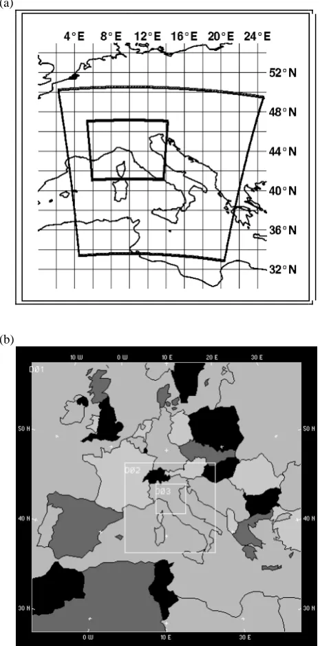
The non-hydrostatic COSMO and MM5 limited-area models are used to perform the meteorological simulations. Table 1 briefly summarizes the different models’ experiments, with their main characteristics such as initial and boundary con-ditions, the nesting technique, the number of vertical levels and the models’ horizontal resolutions. The model integra-tion domains are shown in Fig. 5.
4.1 COSMO model
The COSMO model (previously known as Lokal Modell) was originally developed at the DWD (Deutscher WetterDi-enst) (Steppeler et al., 2003) and it is currently developed and maintained by the COSMO Consortium (COnsortium for Small-scale Modelling), which involves Germany, Italy, Switzerland, Greece, Poland and Romania.
COSMO is a non-hydrostatic model, based on the primi-tive equations describing fully compressible non-hydrostatic flow in a moist atmosphere, without any scale approxima-tion. The model equations are expressed with 5 prognostic variables: temperature, pressure, humidity, horizontal and vertical velocity components. They are solved numerically using the traditional finite difference method on a Arakawa-C grid. In the vertical, a terrain following hybrid sigma-type coordinate is used. The subgrid-scale physical processes de-scribed by parameterisation schemes are: radiation (Ritter-Geleyn, 1992, scheme), surface turbulent fluxes and verti-cal diffusion, soil processes, subgrid-sverti-cale clouds, moist con-vection (Tiedtke, 1989, mass-flux scheme), grid-scale clouds and precipitation. The microphysical scheme includes 5 hy-drometeors, for which the prognostic equations are solved: cloud ice, cloud water, rain, snow, graupel. For a com-plete description of the model, the reader is referred to the COSMO web site (http://www.cosmo-model.org/, mirror site on http://cosmo-model.cscs.ch/).
ARPA-SIM has been using COSMO as the operational forecast model since 2001; COSMO is run twice a day (at 00:00 UTC and 12:00 UTC) for 72 h with a spatial horizontal resolution of 7 km and 40 layers in the vertical. The bound-ary conditions are supplied (one-way nesting) by the global model of the ECMWF (European Centre for Medium-range Weather Forecasts) every three hours. The initial condition is provided by a mesoscale data assimilation based on a nudg-ing technique. The variables which are assimilated are: tem-perature, humidity and wind.
The model is also operational twice a day at 2.8 km, with 45 vertical layers, nested (one-way) on the 7 km runs starting at 00:00 and 12:00 UTC. The forecast range is 48 h.
For this work, the model (version 3.9) has been run in a slightly different configuration, since only 35 vertical layers have been used for both the 7 km and 2.8 km runs. Grau-pel was not available as a prognostic variable in model ver-sion 3.9. Initial and boundary conditions are provided by ECMWF analyses or forecasts for all the models, testing dif-ferent configurations (Table 1). The model integration do-mains are shown in Fig. 5a.
826 A. Amengual et al.: Hydrometeorological simulations and forecast uncertainty
(a)
(b)
Figure 5. (a) Configuration of the domains used for the COSMO simulations with horizontal resolutions of 7 (larger domain) and 2.8 (smallest domain) km and (b) for the MM5 simulations with horizontal resolutions of 22.5, 7.5 and 2.5 km respectively. The Reno river basin is located between 44°-44.5° N and 10.8°-11.4°.
38
Fig. 5. Configuration of the domains used for: (a) the COSMO
simulations with horizontal resolutions of 7 (larger domain) and 2.8 (smallest domain) km and (b) for the MM5 simulations with hori-zontal resolutions of 22.5, 7.5 and 2.5 km respectively. The Reno river basin is located between 44◦−44.5◦N and 10.8◦−11.4◦.
with the nudging technique over the preceding 12 h (referred to as COSMO analysis in Table 1), while the boundary con-ditions are provided every 3 h by the ECMWF operational model forecasts. In the latter case, therefore, a real time fore-cast is simulated. In the 2.8 km runs an explicit representa-tion of the deep convecrepresenta-tion is allowed by switching off the Tiedtke convection scheme. The simulations are 72 h long.
Table 2. Performance of the rain-gauge driven runoff simulations for the 7–10 November 2003 episode and for the HEC-HMS and TOPKAPI hydrological models in terms of NSE efficiency crite-rion, % EV and % EP at Casalecchio flow-gauge.
MODEL NSE % EV % EP
HMS 0.86 13.2 24.9
TOPKAPI 0.77 34.7 21.2
4.2 MM5 model
MM5 is a high-resolution short-range weather forecast model developed by the Pennsylvania State University (PSU) and the National Center for Atmospheric Research (NCAR) (Dudhia, 1993; Grell et al., 1995). Simulations are designed using 24 verticalσ-levels, with higher density near the sur-face to better resolve near-ground processes, and three spa-tial domains with 151×151 grid points centered in north-western Italy (Fig. 5b). Their respective horizontal reso-lutions are 22.5, 7.5 and 2.5 km. The interaction between the domains follows a two-way nesting strategy (Zhang and Fritsch, 1986). The second and third domains are used to supply the high-resolution rainfall fields to drive the hy-drologic simulations depending on the runoff experiment. With the 2.5 km resolution driving data it is possible to test whether the enhanced representation of local topographic forcings leads to an improvement of the simulated precipi-tation fields.
To parameterise moist convection effects in the meteoro-logical simulations, the modified Kain-Fritsch scheme (Kain and Fritsch, 1993) is used for the first and second domains. In the third domain, the convection is explicitly resolved ow-ing to the very high-resolution. Moist microphysics is rep-resented with prediction equations for cloud and rain water fields, cloud ice and snow allowing for slow melting of snow, supercooled water, graupel and ice number concentration (Reisner et al., 1998). The planetary boundary layer physics is formulated using a modified version of the Hong and Pan scheme (Hong and Pan, 1996). Surface temperature over land is calculated using a force-restore slab model (Black-adar, 1979; Zhang and Anthes, 1982) and over sea it remains constant during the simulations. Finally, long and short wave radiative processes are formulated using the RRTM scheme (Mlawer et al., 1997).
To initialize the model and to provide the boundary conditions, ECMWF (European Centre for Medium-range Weather Forecasts) analyses and forecasts are used depend-ing on the experiment (Table 1). These fields are provided at a spatial resolution of 0.3◦and the update frequency for the boundary conditions is 6 h. The tendencies along the bound-aries of the coarse domain model, specified by differences of the fields between the 6 h apart data, are applied using a New-tonian relaxation approach (Grell et al., 1995). For the MM5
Table 3. Contingency table of possible events for a selected thresh-old.
Observed precipitation
Yes No
Forecasted precipitation Yes a b
No c d
hind+obs at 7.5 (control) and 2.5 km experiments, the first
guess fields – interpolated from the ECMWF analyses on the MM5 model grid – are improved using surface and upper-air observations with a successive-correction objective analysis technique (Benjamin and Seaman, 1985). The whole set of MM5 simulations comprise a 48 h simulation period starting at 12:00 UTC on 7 November 2003.
5 Results and discussion
5.1 Runoff simulations driven by rain-gauge data
The stream-flow simulations are first driven by precipita-tion observaprecipita-tions to be aware of the performance of both rainfall-runoff models. These rain-gauge driven flows will be used, instead of the observed discharge, for the compari-son with the results derived from the meteorological models (Sect. 5.2). In such a way, the systematic error of the hy-drological models will not affect the comparison. The skill of the resulting runoff simulations is expressed in terms of the Nash-Sutcliffe efficiency criterion (NSE; Nash and Sut-cliffe, 1970). The performance of the runoff simulations is also checked by means of the relative error of total volume at Casalecchio Chiusa flow-gauge, expressed as percentage (% EV). Therefore, % EV>0 and % EV<0 would indicate an over and underestimation of the volume by the model, re-spectively. In addition, the relative error in percentage to the peak discharge has also been calculated (% EP).
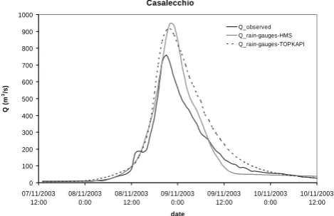
The observed hydrograph depicted a maximum discharge of 757.6 m3s−1 on 21:00 UTC 8 November 2003 (Fig. 6). Rain-gauge driven runoff simulations show a similar perfor-mance in terms of peak runoff for both models, with a no-ticeable overestimation of 160.4 m3s−1and 188.4 m3s−1for TOPKAPI and HEC-HMS, respectively. This represents an overestimation of the observed peak flow slightly above of the 20% for TOPKAPI and very close to 25% for HEC-HMS, respectively. Otherwise, HEC-HMS reproduces the volume and the time base of the observed hydrograph more accu-rately than TOPKAPI. Therefore, NSE and % EV result in a better performance for the former than the latter model (Ta-ble 2 and Fig. 6). The time to peak is identical for both mod-els and it is simulated on 22:00 UTC 8 November 2003 with a delay of only 1 h.
Casalecchio
0 100 200 300 400 500 600 700 800 900 1000
07/11/2003 12:00
08/11/2003 0:00
08/11/2003 12:00
09/11/2003 0:00
09/11/2003 12:00
10/11/2003 0:00
10/11/2003 12:00
date
Q (
m
3/s
)
Q_observed Q_rain-gauges-HMS Q_rain-gauges-TOPKAPI
Figure 6. Rain-gauge driven runoff simulations provided by HEC-HMS and TOPKAPI runoff models versus the observed discharge.
39
Fig. 6. Rain-gauge driven runoff simulations provided by HEC-HMS and TOPKAPI runoff models versus the observed discharge.
The overestimation of the runoff volumes and the peak dis-charges for both models can be ascribed to several factors. First, an inaccurate reproduction of the infiltration processes – that might lead to consider the initial soil moisture content slightly superior to the existent – can produce an overesti-mation of precipitation available for runoff during the event. Second, the presence of a small hydroelectric reservoir lo-cated in the upper catchment – which has not been modeled – can also affect the modeled basin’s response, since its impact on the flow regime and the runoff volume cannot be negligi-ble.
On the other hand, both hydrological models fit the dy-namical routing and the rising limb of the observed hydro-graph quite well, in spite of not reproducing the first bump of runoff observed on 12:00 UTC 8 November 2003. This bump is due to a short intense raining period comprised within the forecast time steps 18th and 21st (Fig. 10), which especially affected the left side of the upper basin. Therefore, this fail-ure could be ascribed to an inaccurate reproduction of the ob-served rainfall field over the area located in the left side of the upper basin, upstream to the Vergato river section (Fig. 4). The scarce presence of rain-gauges in this zone could have affected the accuracy of the rainfall inputs, leading to a slight and localised underestimation of the precipitation amounts.
828 A. Amengual et al.: Hydrometeorological simulations and forecast uncertainty
(a)
9ºE 10ºE 11ºE 12ºE
9ºE 10ºE 11ºE 12ºE
44ºN 45ºN
44ºN 45ºN
1 5 10 20 30 40 50 100
40
(a)
9ºE 10ºE 11ºE 12ºE
9ºE 10ºE 11ºE 12ºE
44ºN 45ºN
44ºN 45ºN
1 5 10 20 30 40 50 100
40
41
41
Figure 7. Observed (a) and forecasted precipitation accumulated over 6 hours (on 12-18 UTC 8 November 2003) provided by the following COSMO runs: (b) control (COSMO hind+obs 7), (c) COSMO hind 7, (d) COSMO fc 7, (e) COSMO hind+obs 2.8, (f) COSMO fc 2.8. Rainfall is shown in mm according to the scale. In Fig. 7a the blue crosses denote the rain-gauges, and the kriged observed precipitation has been blanked in the zones without rain-gauges in order to avoid artificial rainfall distributions.
42
Fig. 7. Observed (a) and forecasted precipitation accumulated over 6 h (on 12:00–18:00 UTC 8 November 2003) provided by the following COSMO runs: (b) control (COSMO hind+obs 7), (c) COSMO hind 7, (d) COSMO fc 7, (e) COSMO hind+obs 2.8, (f) COSMO fc 2.8. Rainfall is shown in mm according to the scale. In Fig. 7a the blue crosses denote the rain-gauges, and the kriged observed precipitation has been blanked in the zones without rain-gauges in order to avoid artificial rainfall distributions.
Despite the abovementioned shortcomings, the reproduc-tion of the flood event provided by both rain-gauge driven hydrological models simulations can be considered accurate, especially from the point of view of stakeholders (i.e. end users such as representatives from civil protection authori-ties for the aims of civil protection), since the timing and the order of magnitude of the event are well simulated.
5.2 Runoff simulations driven by COSMO and MM5 ex-periments
The COSMO and MM5 meteorological simulations have been evaluated at a scale larger than the basin by compar-ing the spatial observed and simulated rainfall accumula-tions over northern Italy in the 6-h period of maximum pre-cipitation (from 12:00 to 18:00 UTC on 8 November 2003; Fig. 7a). Therefore, the analysis of the cumulative rainfall
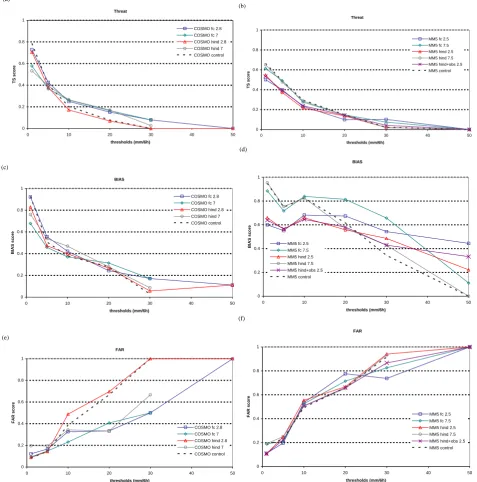
fields for this time window provides valuable information of the models’ skill to simulate the more intense rainfall pe-riod. At this aim, a set of non-parametric statistical scores has been calculated through a point validation methodology. These scores are computed by using a 2×2 contingency table which summarizes in a categorical way the possible com-binations of forecasted and observed events above and be-low a given rainfall threshold (Table 3). Then, Threat Score (TS), Bias Score (BIAS) and False Alarm Ratio (FAR) have been computed according to the following expressions (Jol-liffe and Stephenson, 2003; Wilks, 2006):
TS=a/(a+b+c)
BIAS=(a+b)/(a+c)
FAR=b/(a+b)
Briefly, the threat score indicates the correct proportion for the rainfall threshold being forecasted when it has been re-moved the correct no forecasts. A perfect forecast has TS=1. The bias score is the ratio of the number of positive forecasts to the number of positive observations. Unbiased forecasts exhibit BIAS=1. Finally, the false alarm ratio is the pro-portion of positive forecast events that fail to materialize. A perfect forecast has FAR=0. To interpolate the spatial distri-butions from the models’ grid-points into the 579 rain-gauge point locations available over the domain, it has been used the bilinear interpolation method for each experiment. The set of thresholds includes values up to 50 mm/6 h due to the high intensity of the observed rainfall amounts. It is worth to note that it has not been possible for some experiments to compute statistical scores at the largest thresholds, since the forecasts never exceeded these thresholds.
To quantify the skill of the precipitation fields provided by both COSMO and MM5 simulations at catchment scale, the area-averaged spatial and temporal distributions of these pat-terns are compared against the observed rainfall distribution over the Reno river basin by using two continuous statisti-cal indices: the NSE and the mean absolute error (MAE). At this aim, the 13 subbasins segmentation of the catchment – carried out to implement the HEC-HMS runoff model in its semi-distributed configuration – has been used to evaluate the spatial distributions. Each individual subbasin has been used as an areal accumulation unit for the rainfall amounts over a 48 h time window, starting at 13:00 UTC on 7 Novem-ber 2003. Thus, the results based on these cumulative rain-fall fields provide information of the general performance of the models to simulate the whole event. The temporal distri-butions are computed by using hourly rainfall amounts over the whole basin and during the same 48 h time period. The hourly discretizations are found suitable in order to evalu-ate the ability of the mesoscale models of providing enough intense simulated rainfall fields, owing to the short times of concentration of the basin when it is affected by intense rainfall.
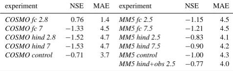
Table 4. NSE efficiency criterion and MAE (in mm) of the spatial area-averaged rainfall distributions yielded by the set of mesoscale numerical simulations.
experiment NSE MAE experiment NSE MAE
COSMO fc 2.8 0.76 1.4 MM5 fc 2.5 −1.15 4.5
COSMO fc 7 −1.33 4.5 MM5 fc 7.5 −1.21 4.5
COSMO hind 2.8 −1.52 4.7 MM5 hind 2.5 −0.83 4.1
COSMO hind 7 −1.53 4.7 MM5 hind 7.5 −0.90 4.2
COSMO control −0.71 3.7 MM5 control −1.00 4.3
MM5 hind+obs 2.5 −0.77 4.0
5.2.1 COSMO and MM5 control runs
Six hourly accumulated precipitations provided by both COSMO and MM5 control simulations over northern Italy are analysed. The COSMO simulation reproduces quite well the precipitation occurred over the north-eastern Alps, even if the structure is spatially shifted (Fig. 7b), whereas the MM5 experiment shows a greater spread in simulating the precip-itation field over the Alps, together with a slight overfore-casting of the rainfall amounts (Fig. 8a). Both models do not forecast correctly the rainfall amounts observed within the Reno river basin, but capture the precipitation pattern over the western part of the Apennines. Therefore, the rainfall amounts inside the catchment are underestimated.
COSMO and MM5 control simulations show the high-est TS value at small thresholds, with TS rapidly decreas-ing for higher thresholds (Fig. 9a and b). For medium and high thresholds, the MM5 control is better than COSMO in terms of TS. Both experiments underforecast the precipita-tion amounts over the whole domain (Fig. 9c and d), but the MM5 simulation presents a better performance with re-spect to COSMO, the MM5 BS being generally closer to 1. Regarding the FAR (Fig. 9e and f), both control experi-ments display a small proportion of incorrect forecasts for the lowest thresholds, but the false alarms increase rapidly for moderate and intense rainfall. At low- and mid-thresholds, the COSMO run is more accurate than the MM5 simula-tion. It seems that the greater rainfall amounts simulated by the MM5 experiment produce more hits but also more false alarms.
It is worth to note that both models are driven by the same initial and boundary conditions and with an assimila-tion of observaassimila-tional data. Therefore, the aforemenassimila-tioned differences can be ascribed to the different model formula-tions and, possibly, to the different physical parameteriza-tions. Maybe the convection scheme of the MM5 model is re-sponsible for the enhancement of the rainfall amounts within this complex orographic area. The higher vertical resolution of the COSMO model does not seem to be beneficial for this case.
830 A. Amengual et al.: Hydrometeorological simulations and forecast uncertainty 1 5 10 20 30 40 50 100
9ºE 10ºE 11ºE 12ºE
45ºN
44ºN 45ºN
44ºN
9ºE 10ºE 11ºE 12ºE
(a) 1 5 10 20 30 40 50 100
9ºE 10ºE 11ºE 12ºE
45ºN
44ºN 45ºN
44ºN
9ºE 10ºE 11ºE 12ºE
(a) 1 5 10 20 30 40 50 100
9ºE 10ºE 11ºE 12ºE
45ºN
44ºN 45ºN
44ºN
9ºE 10ºE 11ºE 12ºE
(b) 1 5 10 20 30 40 50 100
9ºE 10ºE 11ºE 12ºE
45ºN
44ºN 45ºN
44ºN
9ºE 10ºE 11ºE 12ºE
(b) 43 1 5 10 20 30 40 50 100
9ºE 10ºE 11ºE 12ºE
45ºN
44ºN 45ºN
44ºN
9ºE 10ºE 11ºE 12ºE
(a) 1 5 10 20 30 40 50 100
9ºE 10ºE 11ºE 12ºE
45ºN
44ºN 45ºN
44ºN
9ºE 10ºE 11ºE 12ºE
(a) 1 5 10 20 30 40 50 100
9ºE 10ºE 11ºE 12ºE
45ºN
44ºN 45ºN
44ºN
9ºE 10ºE 11ºE 12ºE
(b) 1 5 10 20 30 40 50 100
9ºE 10ºE 11ºE 12ºE
45ºN
44ºN 45ºN
44ºN
9ºE 10ºE 11ºE 12ºE
(b) 43 1 5 10 20 30 40 50 100
9ºE 10ºE 11ºE 12ºE
45ºN
44ºN 45ºN
44ºN
9ºE 10ºE 11ºE 12ºE
(c) 1 5 10 20 30 40 50 100
9ºE 10ºE 11ºE 12ºE
45ºN
44ºN 45ºN
44ºN
9ºE 10ºE 11ºE 12ºE
(c) 9ºE 1 5 10 20 30 40 50 100 12ºE 11ºE 10ºE 45ºN 44ºN 45ºN 44ºN
9ºE 10ºE 11ºE 12ºE
(d) 9ºE 1 5 10 20 30 40 50 100 12ºE 11ºE 10ºE 45ºN 44ºN 45ºN 44ºN
9ºE 10ºE 11ºE 12ºE
(d) 44 1 5 10 20 30 40 50 100
9ºE 10ºE 11ºE 12ºE
45ºN
44ºN 45ºN
44ºN
9ºE 10ºE 11ºE 12ºE
(c) 1 5 10 20 30 40 50 100
9ºE 10ºE 11ºE 12ºE
45ºN
44ºN 45ºN
44ºN
9ºE 10ºE 11ºE 12ºE
(c) 9ºE 1 5 10 20 30 40 50 100 12ºE 11ºE 10ºE 45ºN 44ºN 45ºN 44ºN
9ºE 10ºE 11ºE 12ºE
(d) 9ºE 1 5 10 20 30 40 50 100 12ºE 11ºE 10ºE 45ºN 44ºN 45ºN 44ºN
9ºE 10ºE 11ºE 12ºE
(d) 44 9ºE 1 5 10 20 30 40 50 100 12ºE 11ºE 10ºE 45ºN 44ºN 45ºN 44ºN
9ºE 10ºE 11ºE 12ºE
(e) 9ºE 1 5 10 20 30 40 50 100 12ºE 11ºE 10ºE 45ºN 44ºN 45ºN 44ºN
9ºE 10ºE 11ºE 12ºE
(e) 9ºE 1 5 10 20 30 40 50 100 12ºE 11ºE 10ºE 45ºN 44ºN 45ºN 44ºN
9ºE 10ºE 11ºE 12ºE
(f) 9ºE 1 5 10 20 30 40 50 100 12ºE 11ºE 10ºE 45ºN 44ºN 45ºN 44ºN
9ºE 10ºE 11ºE 12ºE
(f)
Figure 8. Forecasted precipitation accumulated over 6 hours (on 12-18 UTC 8 November 2003)provided by the following MM5 runs: (a) control (MM5 hind+obs 7.5), (b) MM5 hind 7.5, (c) MM5 fc 7.5, (d) MM5 hind+obs 2.5, (e) MM5 hind 2.5 and (f) MM5 fc 2.5. Rainfall is shown in mm according to the scale.
45 9ºE 1 5 10 20 30 40 50 100 12ºE 11ºE 10ºE 45ºN 44ºN 45ºN 44ºN
9ºE 10ºE 11ºE 12ºE
(e) 9ºE 1 5 10 20 30 40 50 100 12ºE 11ºE 10ºE 45ºN 44ºN 45ºN 44ºN
9ºE 10ºE 11ºE 12ºE
(e) 9ºE 1 5 10 20 30 40 50 100 12ºE 11ºE 10ºE 45ºN 44ºN 45ºN 44ºN
9ºE 10ºE 11ºE 12ºE
(f) 9ºE 1 5 10 20 30 40 50 100 12ºE 11ºE 10ºE 45ºN 44ºN 45ºN 44ºN
9ºE 10ºE 11ºE 12ºE
(f)
Figure 8. Forecasted precipitation accumulated over 6 hours (on 12-18 UTC 8 November 2003)provided by the following MM5 runs: (a) control (MM5 hind+obs 7.5), (b) MM5 hind 7.5, (c) MM5 fc 7.5, (d) MM5 hind+obs 2.5, (e) MM5 hind 2.5 and (f) MM5 fc 2.5. Rainfall is shown in mm according to the scale.
45
Fig. 8. Forecasted precipitation accumulated over 6 h (on 12-18 UTC 8 November 2003) provided by the following MM5 runs: (a) control (MM5 hind+obs 7.5), (b) MM5 hind 7.5, (c) MM5 fc 7.5, (d) MM5 hind+obs 2.5, (e) MM5 hind 2.5 and (f) MM5 fc 2.5. Rainfall is shown in mm according to the scale.
and MM5 simulations show a low forecasting skill at small scales. The inaccuracies in correctly forecasting the tim-ing and rainfall amount over the upper Reno river basin are depicted in Figs. 10 and 11. In particular, the experiments miss the highest precipitation amounts observed around the 25th forecast hour. Therefore, the severe underestimation of the maximum precipitation amounts and the wrong tim-ing are propagated to the subsequent driven runoff hydro-graphs (Tables 6 and 7), which exhibit a negative relative
error in total volume. The hydrological runs (Figs. 12 and 13) simulate a discharge value exceeding only the warning threshold (i.e. 80 m3s−1), but not the pre-alarm level (i.e. 630 m3s−1): COSMO-TOPKAPI and COSMO-HEC driven experiments show a maximum peak discharge slightly supe-rior to 275 m3s−1(Fig. 12a and b) and MM5-TOPKAPI and MM5-HEC driven runoff experiments yield maximum dis-charges slightly below 200 m3s−1(Fig. 13a and b).
A. Amengual et al.: Hydrometeorological simulations and forecast uncertainty 831
(a)
Threat
0 0.2 0.4 0.6 0.8 1
0 10 20 30 40
thresholds (mm/6h)
TS score
50 COSMO fc 2.8 COSMO fc 7 COSMO hind 2.8 COSMO hind 7 COSMO control
(b)
Threat
0 0.2 0.4 0.6 0.8 1
0 10 20 30 40 5
thresholds (mm/6h)
TS score
0 MM5 fc 2.5 MM5 fc 7.5 MM5 hind 2.5 MM5 hind 7.5 MM5 hind+obs 2.5 MM5 control
46
0 0.2 0.4 0.6 0.8 1
0 10 20 30 40
thresholds (mm/6h)
TS score
50 COSMO fc 2.8 COSMO fc 7 COSMO hind 2.8 COSMO hind 7 COSMO control
(b)
Threat
0 0.2 0.4 0.6 0.8 1
0 10 20 30 40 5
thresholds (mm/6h)
TS score
0 MM5 fc 2.5 MM5 fc 7.5 MM5 hind 2.5 MM5 hind 7.5 MM5 hind+obs 2.5 MM5 control
46
(c)
BIAS
0 0.2 0.4 0.6 0.8 1
0 10 20 30 40
thresholds (mm/6h)
BIAS score
50 COSMO fc 2.8 COSMO fc 7 COSMO hind 2.8 COSMO hind 7 COSMO control
(d)
BIAS
0 0.2 0.4 0.6 0.8 1
0 10 20 30 40
thresholds (mm/6h)
BIAS score
50 MM5 fc 2.5
MM5 fc 7.5 MM5 hind 2.5 MM5 hind 7.5 MM5 hind+obs 2.5 MM5 control
47
(c)
BIAS
0 0.2 0.4 0.6 0.8 1
0 10 20 30 40
thresholds (mm/6h)
BIAS score
50 COSMO fc 2.8 COSMO fc 7 COSMO hind 2.8 COSMO hind 7 COSMO control
(d)
BIAS
0 0.2 0.4 0.6 0.8 1
0 10 20 30 40
thresholds (mm/6h)
BIAS score
50 MM5 fc 2.5
MM5 fc 7.5 MM5 hind 2.5 MM5 hind 7.5 MM5 hind+obs 2.5 MM5 control
47
(e)
FAR
0 0.2 0.4 0.6 0.8 1
0 10 20 30 40 5
thresholds (mm/6h)
FAR score
0 COSMO fc 2.8 COSMO fc 7 COSMO hind 2.8 COSMO hind 7 COSMO control
(f)
FAR
0 0.2 0.4 0.6 0.8 1
0 10 20 30 40 5
thresholds (mm/6h)
FAR score
0 MM5 fc 2.5 MM5 fc 7.5 MM5 hind 2.5 MM5 hind 7.5 MM5 hind+obs 2.5 MM5 control
Figure 9. TS, BIAS and FAR skill scores for different 6-h rainfall amount thresholds
obtained by the COSMO and MM5 meteorological experiments.
48
Fig. 9. TS, BIAS and FAR skill scores for different 6-h rainfall amount thresholds obtained by the COSMO and MM5 meteorological experiments.
5.2.2 COSMO and MM5 experimental runs
Following the motivation and methodology explained in the previous sections, a set of additional experiments is per-formed in order to produce the experimental meteorological model runs. Figures 7 and 8 show the observed and the sim-ulated rainfall accumulations for the remaining COSMO and MM5 experiments over the 6-h period of maximum precipi-tation.
(a) The COSMO based experiments
All the COSMO runs reproduce the observed rainfall struc-ture over the Apennines but underestimate the amounts, es-pecially on the lee side over the Reno river basin (Fig. 7c– f). The tendency to overestimate the rainfall in upwind areas in presence of a mountain range, with a related drying ef-fect in the downwind regions, in case of intense precipitation forecast, has already been recognised as a typical feature of
832 A. Amengual et al.: Hydrometeorological simulations and forecast uncertainty (a) 0 2 4 6 8 10 12
1 3 5 7 9 11 13 15 17 19 21 23 25 27 29 31 33 35
forecast time step
p (mm)
observed COSMO fc 2.8 COSMO fc 7 COSMO hind 2.8 COSMO hind 7 COSMO control 0 20 40 60 80 100
0 5 10 15 20 25 30 35 40 45
forecast time step
cu mul a ti ve hour ly a re al -ave ra ge pr ec ip it at io n ( m m ) observed COSMO 2.8 fc COSMO 7 fc COSMO 2.8 hind COSMO 7 hind COSMO control (b) 0 20 40 60 80 100
0 5 10 15 20 25 30 35 40 45
forecast time step
cu mul a ti ve hour ly a re al -ave ra ge pr ec ip it at io n ( m m ) observed COSMO 2.8 fc COSMO 7 fc COSMO 2.8 hind COSMO 7 hind COSMO control
(b)
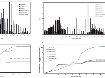
Figure 10. (a) Observed and forecasted hourly areal-averaged amounts and (b) cumulative hourly areal-averaged amounts over the upper Reno river basin provided by the different configurations of COSMO model are displayed from 1300 UTC 7 November 2003 until 00 UTC 09 November 2003
49 (a) 0 2 4 6 8 10 12
1 3 5 7 9 11 13 15 17 19 21 23 25 27 29 31 33 35
forecast time step
p (mm)
observed COSMO fc 2.8 COSMO fc 7 COSMO hind 2.8 COSMO hind 7 COSMO control 0 20 40 60 80 100
0 5 10 15 20 25 30 35 40 45
forecast time step
cu mul a ti ve hour ly a re al -ave ra ge pr ec ip it at io n ( m m ) observed COSMO 2.8 fc COSMO 7 fc COSMO 2.8 hind COSMO 7 hind COSMO control (b) 0 20 40 60 80 100
0 5 10 15 20 25 30 35 40 45
forecast time step
cu mul a ti ve hour ly a re al -ave ra ge pr ec ip it at io n ( m m ) observed COSMO 2.8 fc COSMO 7 fc COSMO 2.8 hind COSMO 7 hind COSMO control
(b)
Figure 10. (a) Observed and forecasted hourly areal-averaged amounts and (b) cumulative hourly areal-averaged amounts over the upper Reno river basin provided by the different configurations of COSMO model are displayed from 1300 UTC 7 November 2003 until 00 UTC 09 November 2003
49
Fig. 10. (a) Observed and forecasted hourly area-averaged amounts and (b) cumulative hourly area-averaged amounts over the up-per Reno river basin provided by the different configurations of COSMO model are displayed from 13:00 UTC 7 November 2003 until 00:00 UTC 09 November 2003.
the COSMO model (Elementi et al., 2005). This drawback heavily influences the reliability of the meteo-hydrological forecasting chain implemented for the concerned watershed, resulting in an underestimation of the forecast streamflow (Diomede et. al, 2008). In fact, being located on the north-eastern side of the Apennine barrier, the Reno river basin clearly suffers from such a problem when the flow is from the south-west quadrant.
On the contrary, the precipitation occurred over the Alps is forecasted quite well in terms of rainfall amounts and their spatial distribution (Fig. 7c–f). In general, high-resolution experiments produce highest amounts of rainfall for this pe-riod; the best forecast is provided by the COSMO fc 2.8 run (Fig. 7f). This simulation reproduces the whole rainfall struc-ture quite well within the Reno river basin, but only forecasts moderate amounts of rain.
With regard to the Threat Score (Fig. 9a), COSMO high-resolution experiments show the highest value at the smallest threshold. At the higher thresholds, no benefits are obtained by the high-resolution runs: COSMO hind 2.8 has the lower score, while COSMO fc 2.8 has a similar behaviour to the 7 km runs. The underforecasting of the precipitation amounts over northern Italy, expressed by the BS (Fig. 9c), remains uncorrected, since no significant differences can be found
(a) 0 2 4 6 8 10 12
1 3 5 7 9 11 13 15 17 19 21 23 25 27 29 31 33 35
forecast time step
p (mm)
observed MM5 fc 2.5 MM5 fc 7.5 MM5 hind 2.5 MM5 hind 7.5 MM5 hind+obs 2.5 MM5 control 0 20 40 60 80 100
0 5 10 15 20 25 30 35 40 45
forecast time step
cum u la ti ve hou rl y ar eal -a ver age pr e c ip it at ion (m m ) observed MM5 fc 2.5 MM5 fc 7.5 MM5 hind 2.5 MM5 hind 7.5 MM5 hind+obs 2.5 MM5 control (b) 0 20 40 60 80 100
0 5 10 15 20 25 30 35 40 45
forecast time step
cum u la ti ve hou rl y ar eal -a ver age pr e c ip it at ion (m m ) observed MM5 fc 2.5 MM5 fc 7.5 MM5 hind 2.5 MM5 hind 7.5 MM5 hind+obs 2.5 MM5 control
(b)
Figure 11. (a) Observed and forecasted hourly areal-averaged amounts and (b) cumulative hourly areal-averaged amounts over the upper Reno river basin provided by the different configurations of MM5 model are displayed from 1300 UTC 7 November 2003 until 00 UTC 09 November 2003
50 (a) 0 2 4 6 8 10 12
1 3 5 7 9 11 13 15 17 19 21 23 25 27 29 31 33 35
forecast time step
p (mm)
observed MM5 fc 2.5 MM5 fc 7.5 MM5 hind 2.5 MM5 hind 7.5 MM5 hind+obs 2.5 MM5 control 0 20 40 60 80 100
0 5 10 15 20 25 30 35 40 45
forecast time step
cum u la ti ve hou rl y ar eal -a ver age pr e c ip it at ion (m m ) observed MM5 fc 2.5 MM5 fc 7.5 MM5 hind 2.5 MM5 hind 7.5 MM5 hind+obs 2.5 MM5 control (b) 0 20 40 60 80 100
0 5 10 15 20 25 30 35 40 45
forecast time step
cum u la ti ve hou rl y ar eal -a ver age pr e c ip it at ion (m m ) observed MM5 fc 2.5 MM5 fc 7.5 MM5 hind 2.5 MM5 hind 7.5 MM5 hind+obs 2.5 MM5 control
(b)
Figure 11. (a) Observed and forecasted hourly areal-averaged amounts and (b) cumulative hourly areal-averaged amounts over the upper Reno river basin provided by the different configurations of MM5 model are displayed from 1300 UTC 7 November 2003 until 00 UTC 09 November 2003
50
Fig. 11. (a) Observed and forecasted hourly area-averaged amounts and (b) cumulative hourly area-averaged amounts over the up-per Reno river basin provided by the different configurations of MM5 model are displayed from 13:00 UTC 7 November 2003 until 00:00 UTC 09 November 2003.
Table 5. NSE efficiency criterion and MAE (in mm) of the temporal area-averaged rainfall distributions yielded by the set of mesoscale numerical simulations.
experiment NSE MAE experiment NSE MAE
COSMO fc 2.8 −0.11 1.6 MM5 fc 2.5 −0.58 2.0
COSMO fc 7 −0.30 1.7 MM5 fc 7.5 −0.53 1.9
COSMO hind 2.8 −0.80 2.1 MM5 hind 2.5 −0.55 1.9
COSMO hind 7 −0.92 2.3 MM5 hind 7.5 −0.52 1.9
COSMO control −0.46 1.7 MM5 control −0.54 1.9
MM5 hind+obs 2.5 −0.58 1.9
among the different runs. The False Alarm Ratio is small at the lowest thresholds for all the experiments (Fig. 9e). At increasing thresholds, COSMO hind 2.8 has the worst perfor-mance, while COSMO fc 2.8 has a similar behaviour to the 7 km runs.
At the catchment scale, all the COSMO experiments miss the high precipitation amounts observed around the 25th forecast hour (Fig. 10a). However, the COSMO fc 2.8 exper-iment provides an underestimation of only about 10% for the total areal amount (Fig. 10b), even if this forecast is charac-terised by a wrong temporal distribution. Tables 4 and 5 con-firm that this experiment exhibits the best forecasting skill in terms of NSE and MAE scores among all the COSMO runs.
Table 6. NSE efficiency criterion and percentage of error in volume for the COSMO driven stream-flow experiments performed by the two hydrological models.
Experiment TOPKAPI HEC-HMS
NSE % EV NSE % EV
COSMO fc 2.8 0.58 −21.9 0.51 −21.4
COSMO fc 7 −0.13 −74.4 −0.10 −71.0
COSMO hind 2.8 −0.40 −77.9 −0.19 −72.6
COSMO hind 7 −0.41 −75.5 −0.23 −70.2
COSMO control 0.15 −65.6 0.05 −63.8
The aforementioned inaccuracies of the COSMO simula-tions are propagated to the subsequent set of driven runoff simulations. Figure 12 depicts that the amplitudes of the simulated peaks are considerable smaller than the rain-gauge driven maximum discharge, except for the COSMO fc 2.8 driven experiment. For this experiment, a suitable reproduc-tion can be pointed out for both HEC-HMS and TOPKAPI runs in terms of the peak flows and runoff volumes, although the time to peak is not well fitted. These features are reflected in their statistical scores (Table 6), the COSMO fc 2.8 driven experiments having the smallest values of relative error in volume. Therefore, it is worth to note the usefulness of the
COSMO fc 2.8 driven experiment for the aims of civil
pro-tection: the exceeding of the pre-alarm threshold is forecast correctly, and the delay in the time to peak is not crucial with respect to the forecasting lead time.
(b) The MM5 based experiments
The maximum cumulative values for the MM5 experiments, in terms of precipitation over northern Italy, range from 66 to 93 mm/6 h. However, the highest values – rather similar to the observations – do not lie inside the basin, but westwards of the catchment in the Apennine range. The precipitation amounts occurred over the eastern part of the Alps are also well simulated, even if all the runs forecast excessive quanti-ties over the western and the central Alps (Fig. 8b–f).
Threat Score shows a better performance for the low-resolution simulations at small- and mid-thresholds (Fig. 9b). At the greater thresholds, higher TS is obtained by the high-resolution experiments, owing to the forecasting of higher rainfall amounts. It is worth to note that low-resolution ex-periments presents very similar TS values: it appears that the simulated rainfall patterns are rather insensitive to the dif-ferent initial and boundary conditions used to initialize the MM5 experiments, at least in terms of this index. This fea-ture can be a consequence of dealing with such complex oro-graphic area. In addition, it seems clear that once the low-resolution simulations misplace the correct locations of the precipitation, the high-resolution experiments do not correct these errors due to the two-way nesting strategy.
Casalecchio
0 200 400 600 800 1000
0 12 24 36 48 60 7
forecast time step
Q (
m
3/s
)
2 observed
raingauges
COSMO 2.8 fc COSMO 7 fc
COSMO 2.8 hind
COSMO 7 hind
COSMO control
(a) Casalecchio
0 200 400 600 800 1000
0 12 24 36 48 60 7
forecast time step
Q (
m
3/s
)
2 observed
raingauges
COSMO 2.8 fc COSMO 7 fc
COSMO 2.8 hind
COSMO 7 hind
COSMO control (a)
Casalecchio
0 200 400 600 800 1000
0 12 24 36 48 60 7
forecast time step
Q (
m
3/s
)
2 observed raingauges
COSMO 2.8 fc COSMO 7 fc COSMO 2.8 hind COSMO 7 hind
COSMO control
(b) Casalecchio
0 200 400 600 800 1000
0 12 24 36 48 60 7
forecast time step
Q (
m
3/s
)
2 observed raingauges
COSMO 2.8 fc COSMO 7 fc COSMO 2.8 hind COSMO 7 hind
COSMO control (b)
Figure 12. (a) TOPKAPI and (b) HEC-HMS runoff simulations driven by the different configurations of COSMO, evaluated at Casalecchio outlet.
51
Casalecchio
0 200 400 600 800 1000
0 12 24 36 48 60 7
forecast time step
Q (
m
3/s
)
2 observed raingauges COSMO 2.8 fc COSMO 7 fc COSMO 2.8 hind COSMO 7 hind COSMO control
(a) Casalecchio
0 200 400 600 800 1000
0 12 24 36 48 60 7
forecast time step
Q (
m
3/s
)
2 observed raingauges COSMO 2.8 fc COSMO 7 fc COSMO 2.8 hind COSMO 7 hind COSMO control
(a)
Casalecchio
0 200 400 600 800 1000
0 12 24 36 48 60 7
forecast time step
Q (
m
3/s
)
2 observed raingauges COSMO 2.8 fc COSMO 7 fc COSMO 2.8 hind COSMO 7 hind COSMO control
(b) Casalecchio
0 200 400 600 800 1000
0 12 24 36 48 60 7
forecast time step
Q (
m
3/s
)
2 observed raingauges COSMO 2.8 fc COSMO 7 fc COSMO 2.8 hind COSMO 7 hind COSMO control
(b)
Figure 12. (a) TOPKAPI and (b) HEC-HMS runoff simulations driven by the different configurations of COSMO, evaluated at Casalecchio outlet.
51
Fig. 12. (a) TOPKAPI and (b) HEC-HMS runoff simulations driven by the different configurations of COSMO, evaluated at Casalecchio outlet.
BIAS scores point out an underforecasting of the rain-fall amounts over the whole domain for the MM5 runs, but this feature is more moderate than for the COSMO runs (Fig. 9d). Again, low-resolution predictions outperform the high-resolution forecasts at small thresholds. At medium thresholds, the MM5 fc 7.5 run has the best performance, fol-lowed by the MM5 fc 2.5 run, while at the highest threshold the high-resolution runs perform better, since they provide higher rainfall amounts. FAR values indicate small differ-ences among the low- and high-resolution experiments, and the expected continuous rise of the number of false alarms at increasing thresholds is found (Fig. 9f).