Forecasting Enrollment Based On The Number Of Recurrences Of Fuzzy Relationships And K-means Clustering

Vol. 3 Issue 4, April - 2017

Forecasting Enrollment Based on the Number

of Recurrences of Fuzzy Relationships and

K-Means Clustering

Nghiem Van Tinh

Thai Nguyen University of Technology, Thai Nguyen University Thainguyen, Vietnam

Abstract—In our daily life, people often use

forecasting method to forecast real problems, such as forecasting stock markets, forecasting enrolments, temperature prediction, population growth prediction, etc. Most of the forecasting approaches based on fuzzy time series used the static length of intervals (i.e, the same length of intervals). The disadvantage of the static length of intervals is that the historical data are roughly put into intervals, although the variance of the them is not high. In this paper, a new forecasting model based on combining the Fuzzy Time Series (FTS) and K-mean clustering algorithm with two computational methods, the recurrent fuzzy

relationship groups (RFRG) and K-mean

clustering technique, is presented for academic enrolments. Firstly, we use the K-mean clustering algorithm to divide the historical data into clusters and adjust them into intervals with different lengths. Then, based on the new intervals obtained, we fuzzify all the historical data, identify all fuzzy relationships, construct the recurrent fuzzy logical relationship groups and calculate the forecasted output by the proposed method. Finally, the 22 years of enrollment of Alabama is used to verify the feasibility of the model. Compared to the other methods existing, particularly to the first-order FTS and the high order- FTS, the proposed method showed a better accuracy in forecasting the number of students of the University of Alabama from 1971s to 1992s.

Keywords— Fuzzy time series(FTS), Recurrent fuzzy relations (RFRs), forecasting, K-mean clustering, enrollments.

I. INTRODUCTION

Future prediction of time series events has attracted people from the beginning of times. They used some forecasting models to deal with various problems: such as the enrolment forecasting [2], [4], [11], crop forecast [7], [8], Temperature prediction [14], [20], [21] , stock markets [14], etc. There is the matter of fact that the traditional forecasting methods cannot deal with the forecasting problems in which the historical data are represented by linguistic values. Song and Chissom [2], [3] proposed the time-invariant FTS and the time-variant FTS model which use the max–min operations to forecast the enrolments of the

University of Alabama. However, the main drawback of these methods is huge computation weight when a fuzzy relationship matrix is large. Then, Chen [4] proposed the first-order FTS

model which used the first-order fuzzy relationship groups (FRGs) to simplify the computational complexity of the forecasting process. His model employed simple arithmetic calculations instead of max-min composition operations for better forecasting accuracy. Afterward, fuzzy time series has been widely studied to improve the accuracy of forecasting in many applications. Huarng [6] presented a method for forecasting the enrolments of the University of Alabama and the TAIFEX based on [4] by adding a heuristic function to get better forecasting results. Chen also extended his previous work to present several forecast models based on the high-order fuzzy time series to deal with the enrolments forecasting problem [9], [12]. Yu shown models of refinement relation [5] and weighting scheme [10] for improving forecasting accuracy. Both the stock index and enrolment are used as the targets in the empirical analysis. Ref.[13] presented a new forecast model based on the trapezoidal fuzzy numbers. Huarng [19] shown that different lengths of intervals may affect the accuracy of forecast. He modified previous method by using the ratio-based length to get better forecasting accuracy. Recently, in [17], [20] a new hybrid forecasting model which combined particle swarm optimization with FTS to find proper length of each interval and adjust interval lengths. Some other techniques for determining best intervals and interval lengths based on clustering techniques are found in [15], [16], [18], [23].

Vol. 3 Issue 4, April - 2017

The remainder of this paper is organized as follows. In Section II, we provide a brief review of FTS and K-means clustering algorithm. In Section III, we present a new method for handing forecasting problems based on K-means clustering algorithm through the experiments of forecasting enrolment of the university of Alabama. Then, the experimental results are shown and analyzed in Section IV. Finally, conclusions are presented in Section V.

II.FUZZY TIME SERIES AND K-MEANS ALGORITHM

In this section, we provide briefly some definitions of fuzzy time series in Subsection A and K-mean clustering algorithm in Subsection B.

Fuzzy Time Series

Song and Chissom proposed the definition of FTS [2, 3] based on fuzzy sets. Let U={u1,u2,…,un } be an

universal set; a fuzzy set A of U is defined as A={ fA(u1)/u1+…+fA(un)/un }, where fA is a membership

function of a given set A, fA :U [0,1], fA(ui) indicates the grade of membership of uiin the fuzzy set A, fA(ui)

ϵ [0, 1], and 1≤ i ≤ n . General definitions of fuzzy time series are given as follows:

Definition 1: Fuzzy time series

Let Y(t) (t = ..., 0, 1, 2 …), a subset of R, be the universe of discourse on which fuzzy sets fi(t) (i = 1,2…) are defined and if F(t) be a collection of fi(t)) (i = 1, 2…). Then, F(t) is called a fuzzy time series on Y(t) (t . . ., 0, 1,2, . . .).

Definition 2: Fuzzy logic relationship

If there exists a fuzzy relationship R(t-1,t), such that F(t) = F(t-1) R(t-1,t), where " " is an arithmetic operator, then F(t) is said to be caused by F(t-1). The relationship between F(t) and F(t-1) can be denoted by F(t-1)→ F(t). Let Ai = F(t) and Aj = F(t-1), the relationship between F(t) and F(t -1) is denoted by fuzzy logical relationship Ai→ Aj where Ai and Aj refer to the current state or the left hand side and the next state or the right-hand side of fuzzy time series. Definition 3: 𝝀- order fuzzy time series

Let F(t) be a fuzzy time series. If F(t) is caused by F(t-1), F(t-2),…, F(t-𝜆+1) F(t-𝜆) then this fuzzy relationship is represented by by F(t-𝜆), …, F(t-2), F(t-1)→ F(t) and is called an 𝝀- order fuzzy time series.

Definition 4: Recurrent fuzzy relationship group (RFRG)

Fuzzy logical relationships with the same fuzzy set on the left-hand side can be further grouped into a fuzzy relationship group. Suppose there are relationships such that:

Ai → Ak; Ai → Am; Ai → Ak; …….

So, based on[10], these fuzzy logical relationship can be grouped into the same FRG as : A_i → A_k , A_m, A_k…

K-means clustering technique

K-means clustering introduced in [1] is one of the simplest unsupervised learning algorithms for solving the well-known clustering problem. K-means clustering method groups the data based on their closeness to each other according to Euclidean distance. The main idea of the K-means algorithm is

the minimization of an objective function usually taken up as a function of the deviations between all patterns from their respective cluster centers.

The K-means algorithm can be summarized as:

1. Randomly select cluster centroid vectors to set an initial dataset partition.

2. Assign each document vector to the closest cluster centroids.

3. Recalculate the cluster centroid vector 𝑐𝑗as follows:

𝑐𝑗=_𝑛1

𝑗∑∀𝑑𝑗∈𝑠𝑗𝑑𝑗

4. Repeate step 2 and 3 until the convergence is achieved.

where dj denotes the document vectors that belong to cluster Sj; cj stands for the centroid vector; nj is the number of document vectors that belong to cluster Sj

III. FORECASTING MODEL BASED ON K-MEAN

CLUSTERING AND RFRGS

In this section, we present a new method for forecasting the enrolments of University of Alabama based on recurrent fuzzy relationship groups and K-means clustering algorithm. Firstly, we apply K-K-means clustering algorithm to classify the collected data into clusters and adjust these clusters into contiguous intervals in the generating interval stage from the enrolment data in Subsection A. Then, from the defined interval, we fuzzify on the historical data, determine fuzzy relationships and establish recurrent fuzzy relationship groups. Finally, we obtain the forecasting output based on the recurrent fuzzy relationship groups and rules of forecasting output are our proposed in Subsection B. To verify the effectiveness of the proposed model, all historical enrolments [4] are used to illustrate the first - order fuzzy time series forecasting process shown in Table 1.

TABLE I: HISTORICAL DATA OF ENROLMENTS

Year Actual Year Actual

1971 13055 1982 15433

1972 13563 1983 15497

1973 13867 1984 15145

1974 14696 1985 15163

1975 15460 1986 15984

1976 15311 1987 16859

1977 15603 1988 18150

1978 15861 1989 18970

1979 16807 1990 19328

1980 16919 1991 19337

1981 16388 1992 18876

Source: In [2-4]

The K-mean Clustering Algorithm For Generating Intervals From Historical Data Of Enrolments.

Vol. 3 Issue 4, April - 2017 {13055}, {13563}, {13867}, {14696,15145,15163},

{15311},{15433,15460,15497},{15603},{15861,15984}, {16388}, {16807}, {16859}, {16919}, {18150}, {18876, 18970,19328,19337}

Step 2: Calculate the cluster center

In this step, we use automatic clustering techniques [18] to generate cluster center (Centerk) from clusters according to (1)as follows:

Centerk= ∑ni=1di

n (1)

where di is a datum in clusterk , n denotes the number of data in clusterk and 1 ≤ 𝑘 ≤ 𝑞.

Step 3: Adjust the clusters into intervals according to the follow rules.

Assume that Centerk and Centerk+1 are adjacent cluster centers, then the upper bound Cluster _ UBkof clusterkand the lower bound cluster_LBk+1of clusterk+1

can be calculated as follows:

𝐶𝑙𝑢𝑠𝑡𝑒𝑟_𝑈𝐵𝑘=𝐶𝑒𝑛𝑡𝑒𝑟𝑘+ 𝐶𝑒𝑛𝑡𝑒𝑟𝑘+1₂ (2)

𝐶𝑙𝑢𝑠𝑡𝑒𝑟_𝐿𝐵_𝑘+1= 𝐶𝑙𝑢𝑠𝑡𝑒𝑟_𝑈𝐵_𝑘 (3) where k = 1,.., q-1. Because there is no previous cluster before the first cluster and there is no next cluster after the last cluster, the lower bound Cluster _ LB1 of the first cluster and the upper bound Cluster _ UBqof the last cluster can be calculated as follows:

𝐶𝑙𝑢𝑠𝑡𝑒_𝐿𝐵1= 𝐶𝑒𝑛𝑡𝑒𝑟1− (𝐶𝑒𝑛𝑡𝑒𝑟1− 𝐶𝑙𝑢𝑠𝑡𝑒𝑟_𝑈𝐵1 ) (4)

𝐶𝑙𝑢𝑠𝑡𝑒_𝑈𝐵_𝑝 = 𝐶𝑒𝑛𝑡𝑒𝑟_𝑞+ (𝐶𝑒𝑛𝑡𝑒𝑟_𝑝− 𝐶𝑙𝑢𝑠𝑡𝑒𝑟_𝐿𝐵_𝑞) (5)

Step 4: Let each cluster Cluster_𝑘 form an interval 𝑖𝑛𝑡𝑒𝑟𝑣𝑎𝑙𝑘 , which means that the upper bound

𝐶𝑙𝑢𝑠𝑡𝑒𝑟_𝑈𝐵_𝑘 and the lower bound 𝐶𝑙𝑢𝑠𝑡𝑒𝑟_𝐿𝐵_𝑘the cluster 𝑐𝑙𝑢𝑠𝑡𝑒𝑟𝑘 are also the upper bound

𝑖𝑛𝑡𝑒𝑟𝑣𝑎𝑙_𝑈𝐵𝑜𝑢𝑛𝑑𝑘 and the lower bound

𝑖𝑛𝑡𝑒𝑟𝑣𝑎𝑙_𝐿𝐵𝑜𝑢𝑛𝑑_𝑘 of the interval 𝑖𝑛𝑡𝑒𝑟𝑣𝑎𝑙_𝑘 , respectively. Calculate the middle value 𝑀𝑖𝑑_𝑣𝑎𝑙𝑢𝑒𝑘 of

the interval 𝑖𝑛𝑡𝑒𝑟𝑣𝑎𝑙𝑘as follows:

𝑀𝑖𝑑_𝑣𝑎𝑙𝑢𝑒_𝑘=𝑖𝑛𝑡𝑒𝑟𝑣𝑎𝑙_𝐿𝐵𝑘+ 𝑖𝑛𝑡𝑒𝑟𝑣𝑎𝑙_𝑈𝐵𝑘

2 (6)

where 𝑖𝑛𝑡𝑒𝑟𝑣𝑎𝑙_𝐿𝐵𝑜𝑢𝑛𝑑𝑘 and 𝑖𝑛𝑡𝑒𝑟𝑣𝑎𝑙_𝑈𝐵𝑜𝑢𝑛𝑑𝑘 are

the lower bound and the upper bound of the interval 𝑖𝑛𝑡𝑒𝑟𝑣𝑎𝑙_𝑘, respectively, with k = 1,..,q.

Enrolment Forecasting model based on the first-order FTS.

In this section, we present a new method for forecasting enrolments based on the K-mean clustering algorithm and recurrent fuzzy relationship groups. The proposed method is now presented as follows:

Step 1: Partition the universe of discourse U into intervals.

After applying the procedure K-mean clustering, we can get the following 14 intervals and calculate the middle value of the intervals are listed in Table 2.

TABLE II:THE MIDPOINT OF EACH INTERVAL UJ(1 ≤ 𝑗 ≤ 14)

No Intervals MidPoint No Intervals MidPoint

1

[12801,

13309] 13055 8

[15762.5,

16155] 15958.75

2

[13309,

13715] 13512 9

[16155,

16597.5] 16376.25

3

[13715,

14434] 14074.5 10

[16597.5,

16833] 16715.25

4

[14434,

15156] 14795 11

[16833,

16889] 16861

5

[15156,

15387] 15271.5 12

[16889,

17534.5] 17211.75

6

[15387,

15533] 15460 13

[17534.5,

18639] 18086.75

7

[15533,

15762.5] 15647.75 14

[18639,

19617] 19128

Step 2: Define the fuzzy sets (𝐴_𝑖) and fuzzify all historical data

Define each fuzzy set 𝐴𝑖based on the new obtained

14 intervals in step 1 and the historical enrolments shown in Table 1. For 14 intervals, there are 14 linguistic variables Ai (1≤ 𝑖 ≤ 14). For example, 𝐴₁＝ {very very very very few }, 𝐴₂＝{very very very few}, 𝐴3＝{very very few}, 𝐴4＝{very few }, 𝐴5 ＝{few}, 𝐴6

＝{moderate}, 𝐴₇＝{many}, 𝐴₈＝{many many}, 𝐴₉＝ {very many}, 𝐴₁₀＝{too many}, 𝐴₁₁＝{too many many}, 𝐴12＝{too many many many}, 𝐴13＝{too many many

many many} and 𝐴₁₄＝{too many many many many many}. Each linguistic variable represents a fuzzy set by using equation (7). Each historical value is fuzzified according to its highest degree of membership. If the highest degree of belongingness of a certain historical time variable, say F(t−1) occurs at fuzzy set Ai, then F(t−1) is fuzzified as Ai

A₁ = 1

𝑢1+

0.5

𝑢2+

0

𝑢3+ ⋯ +

0

𝑢14

A₂ =0.5

𝑢1+

1

𝑢2+

0.5 𝑢3+ ⋯ +

0

𝑢14

--- A₁₄ = 0

𝑢1+

0

𝑢2+ ⋯ +

0.5

𝑢13+

1

𝑢14

For simplicity, the membership values of fuzzy set Ai

either are 0, 0.5 or 1, where1 ≤ i ≤ 14. The value 0, 0.5 and 1 indicate the grade of membership of uj in the fuzzy set Ai.

The way to fuzzify a historical data is to find the interval it belongs to and assign the corresponding linguistic value to it and finding out the degree of each data belonging to each A_i . If the maximum membership of the historical data is under Ai , then

the fuzzified historical data is labeled as A_i.

For example, the historical enrolment of year 1975 is 15460 which falls within u4 = (14434, 15156], so it belongs to interval u4. Based on Eq. (7), the highest membership degree of A4 occurs at u4 is 1, the historical time variable F(1975) is fuzzified as A4. In the same way, we can complete fuzzified results of the enrolments are listed in Table 3, where all historical data are fuzzified to be fuzzy sets.

Vol. 3 Issue 4, April - 2017

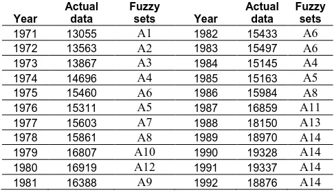
TABLE III:FUZZIFIED ENROLMENTS OF THE UNIVERSITY OF ALABAMA

Year

Actual data

Fuzzy

sets Year

Actual data

Fuzzy sets

1971 13055 A1 1982 15433 A6

1972 13563 A2 1983 15497 A6

1973 13867 A3 1984 15145 A4

1974 14696 A4 1985 15163 A5

1975 15460 A6 1986 15984 A8

1976 15311 A5 1987 16859 A11

1977 15603 A7 1988 18150 A13

1978 15861 A8 1989 18970 A14

1979 16807 A10 1990 19328 A14

1980 16919 A12 1991 19337 A14

1981 16388 A9 1992 18876 A14

Let Y(t) be a historical data time series on year t. The purpose of this step is to get a fuzzy time series F(t) on Y(t). Each element of Y(t) is an integer with respect to the actual enrollment. But each element of F(t) is a linguistic value (i.e. a fuzzy set) with respect to the corresponding element of Y(t). For example, in Table 3, Y(1971) = 13055 and F(1971) = A1; Y(1972) = 13563 and F(1972) = A2; Y(1973) = 13867 and F(1973) = A3 and so on.

Step 3: Create all fuzzy logical relationships

Based on Definition 2. To establish a -order fuzzy relationship, we should find out any relationship which has the F(t −), F(t −+ 1), . . . , F(t − 1) → 𝐹(𝑡) , where F(t −), F(t −+ 1), . . . , F(t − 1) and 𝐹(𝑡) are called the current state and the next state, respectively. Then a  - order fuzzy relationship in the training phase is got by replacing the corresponding linguistic values. For example, supposed = 1 from Table 3, a fuzzy relation A1 → A2 is got as F(1971 →

F(1972) . So on, we get the first-order fuzzy relationships are shown in Table 4, where there are 21 relations; the first 20 relations are called the trained patterns, and the last one is called the untrained pattern (in the testing phase). For the untrained pattern, relation 21 has the fuzzy relation A14 → # as it is created by the relation F(1992) → F(1993), since the linguistic value of F(1993)is unknown within the historical data, and this unknown next state is denoted by the symbol ‘#‘

TABLE IV: THE FIRST-ORDER FUZZY LOGICAL RELATIONSHIPS

No Relationships No Relationships

1 A1 → A2 11 A6 → A6

2 A2 → A3 12 A6 → A4

3 A3 → A4 13 A4 → A5

4 A4 → A6 14 A5 → A8

5 A6 → A5 15 A8 → A11

6 A5 → A7 16 A11 → A13

7 A7 → A8 17 A13 → A14

8 A8 → A10 18 A14 → A14

9 A10 → A12 19 A14 → A14

10 A12 → A9 20 A14 → A14

21 A14 → #

Step 4: Establish all fuzzy logical relationship groups In previous studies[4], [12], [17] the repeated FLRs were simply ignored when fuzzy relationships were

established. But, according to the Definition 4, the recurrence fuzzy relations can be used to indicate how the FLR may appear in the future. From this viewpoint and based on Table 4, we can establish all recurrent fuzzy relationship groups are shown in Table 5.

TABLE V:RECURRENT FUZZY RELATIONSHIP GROUPS (RFRGS)

No group At time RFRGs

1 t =1 A1 → A2

2 t =2 A2 → A3

3 t =3 A3 → A4

4 t =4, 14 A4 → A6, A5 5 t =5, 12, 13 A6 → A5, A6, A4 6 t = 6, 15 A5 → A7, A8

7 t = 7 A7 → A8

8 t = 8, 16 A8 → A10, A11

9 t = 9 A10 → A12

10 t =10 A12 → A9

11 t = 11 A9 → A6

12 t= 17 A11 → A13

13 t=18 A13 → A14

14 t =19,20,21 A14 → A14, A14, A14

Step 5: Calculate the forecasting value for all groups In order to calculate the forecast output for all recurrent fuzzy relationship groups, we use [20] for the trained patterns in the training phase and use [17] the untrained patterns in the testing phase.

For the training phase, we can compute all forecast values for recurrence fuzzy relationship groups based on fuzzy sets on the right-hand or next state within the same group. For each group, we divide each corresponding interval of each next state into p sub-regions with equal size, and calculate a forecasted value for each group according to equation (8).

forecasted_output=1

n∑

(mj+submj) 2 n

j=1 (8)

where,

 n is the total number of next states or the total number of fuzzy sets on the right-hand side within the same group.

mj ( 1 ≤ j ≤ n) is the midpoint of interval uj

corresponding to j-th fuzzy set on the right-hand side where the highest level of fuzzy set Aj takes place in these intervals uj.

𝑠𝑢𝑏𝑚_𝑗 is the midpoint of one of p sub-regions corresponding to j-th fuzzy set on the right-hand side where the highest level of Aj occur in this interval.

For the testing phase, we calculate a forecasted value based on Eq.(9), where the symbol 𝑤ℎ means the

highest votes predefined by user, the symbol  is the order of the fuzzy relationship, the symbols 𝑚_𝑡1 and 𝑚_𝑡𝑖 denote the midpoints of the corresponding intervals of the latest past and other past linguistic values in the current state.

𝐹𝑜𝑟𝑒𝑐𝑎𝑡𝑒𝑑𝑓𝑜𝑟#=

(𝑚𝑡1∗𝑤ℎ)+𝑚𝑡2+⋯+𝑚𝑡𝑖+⋯+𝑚𝑡

𝑤ℎ+(−1) ; i=1:

̅̅̅̅̅ ₍₉₎

Vol. 3 Issue 4, April - 2017

TABLE VI: THE COMPLETE FORECASTED VALUES FOR ALL GROUPS

OF THE FIRST-ORDER FUZZY RELATIONS

No group RFRGs Value

1 A1 → A2 13512

2 A2 → A3 13954.66

3 A3 → A4 14795

4 A4 → A6, A5 15346.5

5 A6 → A5, A6, A4 15236.56

6 A5 → A7, A8 15784.12

7 A7 → A8 15893.34

8 A8 → A10, A11 16807.75

9 A10 → A12 17104.16

10 A12 → A9 16376.25

11 A9 → A6 15435.66

12 A11 → A13 18086.75

13 A13 → A14 19128

14 A14 → A14, A14, A14 19182.33

15 A14 → # 19128

Step 6: Generate all fuzzy forecasting rules based on all RFRGs

Based on each group of fuzzy relationships created and relative forecasting values in Step 5, we can create corresponding fuzzy forecasting rules. The if

-then statements are used as the basic format for the fuzzy forecasting rules. Assume a first-order fuzzy forecasting rule Ri is ‘‘if x = A, then y = B’’, the if-part

of the rule ‘‘x = A’’ is termed antecedent and the then-part of the rule ‘‘y = B’’ is termed consequent. For example, if we want to forecast enrolments Y(t) using fuzzy group 1 for the first-order fuzzy time series in Table 6, the fuzzy forecasting rule R₁ is will be ‘‘if 𝐹(𝑡 − 1) = 𝐴1 then Y(t) = 13512.

In the same way, we can get the 14 fuzzy forecasting rules based on 14 groups of the first-order fuzzy relationship, as shown in Table 7.

TABLE VII: THE FUZZY IF-THEN RULES OF THE FIRST-ORDER FUZZY RELATIONSHIP GROUPS

Rules (R) Antecedent Consequent

1 If F(t-1)== A1 Then Y(t) = 13512 2 If F(t-1)== A2 Then Y(t) = 13954.66 3 If F(t-1)== A3 Then Y(t) = 14795 4 If F(t-1)== A4 Then Y(t) = 15346.5 5 If F(t-1)== A5 Then Y(t) = 15789.12 6 If F(t-1)== A6 Then Y(t) = 15236.56 7 If F(t-1)== A7 Then Y(t) = 15893.34 8 If F(t-1)== A8 Then Y(t) = 16807.75 9 If F(t-1)== A9 Then Y(t) = 15435.66 10 If F(t-1)== A10 Then Y(t) = 17104.16 11 If F(t-1)== A11 Then Y(t) = 18086.75 12 If F(t-1)== A12 Then Y(t) = 16376.25 13 If F(t-1)== A13 Then Y(t) =19212 14 If F(t-1)== A14 Then Y(t) =19182.33

Step 7: Forecasting output based on the forecast rules After the forecast rules are created, we can use them to forecast the training and testing data. Suppose we want to forecast the data Y(t), we need to find out a matched forecast rule and get the forecasted value from this rule. If we use the first-order forecast rules listed in Table 7 to forecast the data Y(t), we just

simply find out the corresponding linguistic values of F(t-1) with respect to the data Y(t-1) and then compare them to the matching parts of all forecast rules. Suppose a matching part of a forecast rule is matched, we then get a forecasted value from the forecasting part of this matched forecast rule. For example, if we want to forecast the data Y(1975), it is necessary to find out the corresponding linguistic values of F(1974) with respect to Y(1974) in Table 3 and get the following pattern.

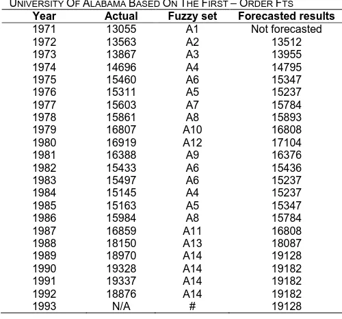
If F(1974) == A3 then forecast Y(1975) = 14795 . In the same way, we complete forecasted output results based on the first - order fuzzy forecast rules in Table 6 are listed in Table 8.

TABLE VIII: THE COMPLETE FORECASTED ENROLMENTS OF

UNIVERSITY OF ALABAMA BASED ON THE FIRST –ORDER FTS

Year Actual Fuzzy set Forecasted results

1971 13055 A1 Not forecasted

1972 13563 A2 13512

1973 13867 A3 13955

1974 14696 A4 14795

1975 15460 A6 15347

1976 15311 A5 15237

1977 15603 A7 15784

1978 15861 A8 15893

1979 16807 A10 16808

1980 16919 A12 17104

1981 16388 A9 16376

1982 15433 A6 15436

1983 15497 A6 15237

1984 15145 A4 15237

1985 15163 A5 15347

1986 15984 A8 15784

1987 16859 A11 16808

1988 18150 A13 18087

1989 18970 A14 19128

1990 19328 A14 19182

1991 19337 A14 19182

1992 18876 A14 19182

1993 N/A # 19128

To evaluate the forecasted performance of proposed method in the fuzzy time series, the mean square error (MSE) is used as an evaluation criterion to represent the forecasted accuracy. The MSE value is calculated according to (10) as follows:

MSE = 1

n∑ (Fi− Ri) 2 n

i= (10)

Where, Ri notes actual data on year i, Fi forecasted value on year i, n is total number of the forecasted data and  is order of the fuzzy relationships.

IV. EXPERIMENTAL RESULTS

In this paper, the proposed method is utilized to forecast the enrolments of University of Alabama with the whole historical data shown in Table 1, the period from 1971 to 1992 are used to perform comparative study in the training and testing phases.

Vol. 3 Issue 4, April - 2017

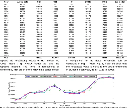
of 20332.67 among all the compared models with the number of intervals of 14; where MSE value is calculated by formula (10) and shown in equation (11). The major difference between the CC06a, HPSO and our models is used in the defuzzification stage and optimization methods. Two models in CC06a [11] and HPSO [17] use the genetic algorithm and the particle swarm optimization algorithm to get the appropriate intervals, respectively, while the proposed model performs the K- mean algorithm to attain the best interval lengths.

Compute forecasting accuracy by MSE values as follows

.

𝑀𝑆𝐸 = ∑𝑁𝑖=1(𝐹𝑖−𝑅𝑖)2

𝑁 =

(13512−13563)2+(13955−13867)2…+(19182−18876)2

21 = 20332.67

where N denotes the number of forecasted data of 21, Fi denotes the forecasted value at time i and Ri denotes the actual value at time i.

TABLE IX: ACOMPARISON OF THE FORECASTED RESULTS BETWEEN OUR MODEL AND THE EXISTING MODELS WITH FIRST-ORDER OF FTS UNDER

DIFFERENT NUMBER OF INTERVALS.

Year Actual data SCI C96 H01 CC06a HPSO Our model

1971 13055 --- --- --- --- --- ---

1972 13563 14000 14000 14000 13714 13555 13512

1973 13867 14000 14000 14000 13714 13994 13955

1974 14696 14000 14000 14000 14880 14711 14795

1975 15460 15500 15500 15500 15467 15344 15347

1976 15311 16000 16000 15500 15172 15411 15237

1977 15603 16000 16000 16000 15467 15411 15784

1978 15861 16000 16000 16000 15861 15411 15893

1979 16807 16000 16000 16000 16831 16816 16808

1980 16919 16813 16833 17500 17106 17140 17104

1981 16388 16813 16833 16000 16380 16464 16376

1982 15433 16789 16833 16000 15464 15505 15436

1983 15497 16000 16000 16000 15172 15411 15237

1984 15145 16000 16000 15500 15172 15411 15237

1985 15163 16000 16000 16000 15467 15344 15347

1986 15984 16000 16000 16000 15467 16018 15784

1987 16859 16000 16000 16000 16831 16816 16808

1988 18150 16813 16833 17500 18055 18060 18087

1989 18970 19000 19000 19000 18998 19014 19128

1990 19328 19000 19000 19000 19300 19340 19182

1991 19337 19000 19000 19500 19149 19340 19182

1992 18876 19000 19000 19149 19014 19014 19182

1993 N/A 19128

MSE 423027 407507 226611 35324 22965 20332.67

Displays the forecasting results of H01 model [5], CC06a model [11], HPSO model [17] and the proposed method. The trend in forecasting of enrolment by first-order of the fuzzy time series model

in comparison to the actual enrolment can be visualized in Fig. 1. From Fig. 1, it can be seen that the forecasted value is close to the actual enrolment of students each year, from 1972s to 1992s.

Fig. 1: The curves of the actual data and the H01, CC06a, HPSO models and our model for forecasting enrolments of University of Alabama

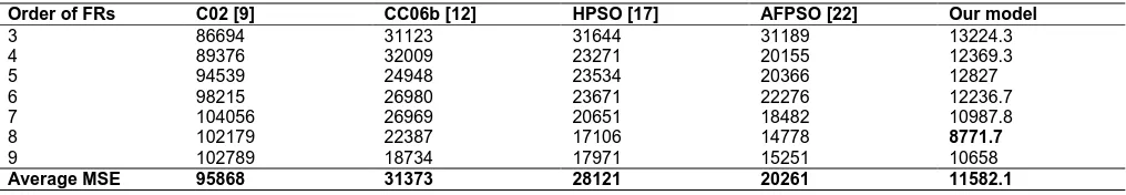
As mentioned above, to verify the forecasting effectiveness for high-order fuzzy time series, five existing forecasting models, the C02 [9], CC06b [12], HPSO [17], AFPSO [22] models are used to compare with the proposed model. A comparison of the forecasted results is listed in Table 10, where the number of intervals is seven for all forecasting models. From Table 10, it is clear that the proposed model is more precise than the other four forecast models at all, since the best and the average fitted accuracies are all the best among the five models.

Practically, at the same intervals, the proposed method obtains the lowest MSE values which are 13224.3, 12369.3, 12827, 12236.7, 10987.8, 8771.7, 10658 for 3-order, 4-order, 5-order, 6-order, 7-order, 8-order and 9-order fuzzy time series, respectively. The proposed model also gets the smallest MSE value of 8771.7 for the 8th-order FTS model. The average MSE value of the proposed model is 11582, which is smallest among all forecasting models compared.

1972 1974 1976 1978 1980 1982 1984 1986 1988 1990 1992

13,000 14,000 15,000 16,000 17,000 18,000 19,000 20,000

Years forecasting

N

um

be

r o

f s

tu

de

nt

s

Vol. 3 Issue 4, April - 2017

TABLE X: A COMPARISON OF THE FORECASTED ACCURACY BETWEEN OUR METHOD AND EXISTING METHODS UNDER VARIOUS HIGH-ORDER FTS MODEL WITH SEVEN INTERVALS

Order of FRs C02 [9] CC06b [12] HPSO [17] AFPSO [22] Our model

3 86694 31123 31644 31189 13224.3

4 89376 32009 23271 20155 12369.3

5 94539 24948 23534 20366 12827

6 98215 26980 23671 22276 12236.7

7 104056 26969 20651 18482 10987.8

8 102179 22387 17106 14778 8771.7

9 102789 18734 17971 15251 10658

Average MSE 95868 31373 28121 20261 11582.1

Experimental results in the testing phase.

To confirm the forecasting accuracy for future enrolments, the historical data of enrolments are separated two parts for independent testing. The first part is used as training data set and the second part is used as the testing data set. In this paper, the historical data of enrolments from year 1971 to 1989 is used as the training data set and the historical data of enrolments from year 1990 to 1992 is used as the testing data set. For example, to forecast a new enrolment of 1990, the enrolments of 1971-1989 are used as the training data. Similarly, a new enrolment of 1991 can be forecasted based on the enrolments

under years 1971-1990. After the training data have been well trained by the proposed model, future enrolments could be obtained to compare with testing data. Some experimental results of the forecasting models for the testing phase are listed in Table 11.

TABLE XI: A COMPARISON OF ACTUAL DATA AND

FORECASTED RESULT FOR SEVEN INTERVALS IN THE TESTINGPHASE

Year Actual data

Forecasted value 1st _-

order 2nd _-

order 3rd _-

order 4th _-

order 5th _-

order 1990 19328 18560 18560 18493 18563 18455 1991 19337 19142 19129 19149 19146 19178 1992 18876 18946 19212 18946 19150 19040

V. CONCLUSION

In this paper, we have proposed a hybrid forecasting model based on fuzzy time series model with recurrent fuzzy relations and K-mean clustering algorithm. By adopting K -mean algorithm, our model can get more suitable partition of the universe of discourse and using recurrence numbers of fuzzy relations, which can improve the forecasting results significantly. The proposed method has been implemented on the historical data of enrolments of University of Alabama to have a comparative study with the existing methods. The detail of comparison was presented in Table 9, 10 and Fig.1. In all cases, the comparison shows that the proposed model outperforms the compared models based on the firs – order FTS and the high – order FTS with different interval lengths. Even the model was only examined in the enrolment forecasting problem; we believe that it can be applied to any other forecasting problems such as population, stock markets, and car road accident forecasting, so on. That will be the future work of this study.

REFERENCES

[1]. J.B. MacQueen, “Some methods for classification and analysis of multivariate observations,” in: Proceedings of the Fifth Symposium on Mathematical Statistics and Probability, vol. 1, University of California Press, Berkeley, CA, pp. 281-297, 1967.

[2]. Q. Song, B.S. Chissom, “Forecasting Enrollments with Fuzzy Time Series – Part I,” Fuzzy set and system, vol. 54, pp. 1-9, 1993b.

[3]. Q. Song, B.S. Chissom, “Forecasting Enrollments with Fuzzy Time Series – Part II,” Fuzzy set and system, vol. 62, pp. 1-8, 1994.

[4]. S.M. Chen, “Forecasting Enrollments based on Fuzzy Time Series,” Fuzzy set and system, vol. 81, pp. 311-319. 1996.

[5]. H.K. Yu, A refined fuzzy time-series model for forecasting, Phys. A, Stat. Mech. Appl. 346, 657– 681,2005;

http://dx.doi.org/10.1016/j.physa.2004.07.024.

[6]. Huarng, K. Heuristic models of fuzzy time series for forecasting. Fuzzy Sets and Systems, 123, 369–386, 2001b .

[7]. Singh, S. R. A simple method of forecasting based on fuzzytime series. Applied Mathematics and Computation, 186, 330–339, 2007a.

[8]. Singh, S. R. A robust method of forecasting based on fuzzy time series. Applied Mathematics and Computation, 188, 472–484, 2007b.

[9]. S. M. Chen, “Forecasting enrollments based on high-order fuzzy time series”, Cybernetics and Systems: An International Journal, vol. 33, pp. 1-16, 2002.

[10]. H.K.. Yu “Weighted fuzzy time series models for TAIEX forecasting ”, Physica A, 349 , pp. 609–624, 2005. [11]. Chen, S.-M., Chung, N.-Y. Forecasting enrollments of

students by using fuzzy time series and genetic algorithms. International Journal of Information and Management Sciences 17, 1–17, 2006a.

[12]. Chen, S.M., Chung, N.Y. Forecasting enrollments using high-order fuzzy time series and genetic algorithms. International of Intelligent Systems 21, 485–501, 2006b.

[13]. Liu, H.T., "An Improved fuzzy Time Series Forecasting Method using Trapezoidal Fuzzy Numbers," Fuzzy Optimization Decision Making, Vol. 6, pp. 63–80, 2007. [14]. Lee, L.-W., Wang, L.-H., & Chen, S.-M. Temperature prediction and TAIFEX forecasting based on fuzzy logical relationships and genetic algorithms. Expert Systems with Applications, 33, 539–550, 2007. [15]. Bulut, E., Duru, O., & Yoshida, S. A fuzzy time series

forecasting model formulti-variate forecasting analysis with fuzzy c-means clustering. WorldAcademy of Science, Engineering and Technology, 63, 765–771, 2012.

Vol. 3 Issue 4, April - 2017 series. Expert Systems with Applications, 36, 2143–

2154, 2009.

[17]. Kuo, I. H., Horng, S.-J., Kao, T.-W., Lin, T.-L., Lee, C.-L., & Pan. An improved method for forecasting enrollments based on fuzzy time series and particle swarm optimization. Expert Systems with applications, 36, 6108–6117, 2009a.

[18]. S.-M. Chen, K. Tanuwijaya, “ Fuzzy forecasting based on high-order fuzzy logical relationships and automatic clustering techniques”, Expert Systems with Applications 38, 15425–15437, 2011.

[19]. Huarng, K.H., Yu, T.H.K., "Ratio-Based Lengths of Intervals to Improve Fuzzy Time Series Forecasting," IEEE Transactions on SMC – Part B: Cybernetics, Vol. 36, pp. 328–340, 2006.

[20]. I-H. Kuo, S.-J. Horng, Y.-H. Chen, R.-S. Run, T.-W. Kao, R.-J. C., J.-L. Lai, T.-L. Lin, Forecasting TAIFEX based on fuzzy time series and particle swarm optimization, Expert Systems with Applications 2(37), (2010) 1494–1502.

[21]. Lee, L.-W. Wang, L.-H., & Chen, S.-M, “Temperature prediction and TAIFEX forecasting based on high order fuzzy logical relationship and genetic simulated annealing techniques”, Expert Systems with Applications, 34, 328–336, 2008b .

[22]. Huang, Y. L., Horng, S. J., He, M., Fan, P., Kao, T. W., Khan, M. K., et al. A hybrid forecasting model for enrollments based on aggregated fuzzy time series and particle swarm optimization. Expert Systems with Applications, 38, 8014–8023, 2011.