Modeling and Analysis of Multi-agent Systems
using Petri Nets
Jose R. Celaya, Alan A. Desrochers, and Robert J. Graves
Email: [email protected], [email protected], and [email protected]
Abstract—The development of theoretical-based methods for the assessment of multi-agent systems properties is of critical importance. This work investigates methodologies for modeling, analysis and design of multi-agent systems. Multi-agent systems are regarded as discrete-event dynamic systems and Petri nets are used as a modeling tool to assess the structural properties of the multi-agent system. Our methodology consists of defining a simple multi-agent system based on the abstract architecture for intelligent agents. The abstract architecture is modeled using Petri nets and structural analysis of the net provides an assessment of the interaction properties of the multi-agent system. Deadlock avoidance in the multi-agent system is considered and it is evaluated using liveness and boundedness properties of the Petri net model.
Index Terms—Petri nets, multi-agent systems, deadlock.
I. INTRODUCTION
Multi-agent systems have been studied for the past few decades. Several multi-agent systems frameworks have been defined in order to apply the multi-agent system con-cept to different applications in control and optimization of complex systems [1]–[4]. An agent is a computer sys-tem or computer program that presents several complex characteristics. The most important characteristic of an agent is that of autonomy. An intelligent agent inhabits an environment and is capable of conducting autonomous actions in order to satisfy its design objective [3], [5]–[7]. An intelligent agent or autonomous agent is an agent that presents some degree of autonomous flexibility by being reactive, pro-active and perhaps sociable [3]. This flexible autonomy is a building block in a multi-agent system. In a multi-agent system, several agents communicate and interact in order to solve a complex problem.
Several interaction frameworks have been defined and they range from collaboration among agents, through competition for resources requiring some level of ne-gotiation in the multi-agent system [3], [7]. In general, the multi-agent system is expected to work properly in a
J. R. Celaya is with the Research Institute for Advanced Computer Science at NASA Ames Research Center, Moffett Field, CA 94035; previously with the Decision Sciences and Engineering Systems De-partment, Rensselaer Polytechnic Institute, Troy, New York 12180.
A. A. Desrochers is with the Electrical, Computer, and Systems Engineering Department, Rensselaer Polytechnic Institute, Troy, New York 12180 (corresponding author phone: 6718; fax: 518-276-8715; e-mail: [email protected]).
R. J. Graves is the Krehbiel Professor of Emerging Technologies, Thayer School of Engineering, Dartmouth College, Hanover, New Hampshire 03755.
dynamic large-scale complex environment (open environ-ment) by having autonomy, adaptability, robustness, and flexibility.
This work presents analytical methodologies for mod-eling and analysis of multi-agent systems. Multi-agent systems are regarded as discrete-event dynamic systems and Petri nets are used as a modeling tool to assess properties of the system.
This document is organized as follows. The problem statement and related work are presented next. Section II presents a brief introduction to multi-agent systems which considers the abstract architecture of intelligent agents, as well as a description of communication and interaction in multi-agent system. Section III presents an introduction to Petri nets. Section IV shows a simple multi-agent system which is modeled with the abstract architecture for intelligent agents as well as Petri nets. Section V presents a methodology to model and analyze multi-agent systems with indirect communication. Finally, section VI discusses the results.
A. Motivation
The complexity and capabilities of a multi-agent system are greater than those presented in distributed software systems. In both cases the study of system properties is becoming more important due to the fact that we are faced more and more with dealing with large complex dynamic systems. Computer simulation is generally used to assess system properties and to verify that the system is achieving its design objectives. An important challenge in this field is the development of analytical methods to assess key properties of such systems [1], [8]. Such methods could be used to provide a preliminary analysis of the multi-agent system, providing design and operation feedback before the development of expensive simulation models.
B. Problem statement
areas for the modeling and analysis of distributed systems [9], flexible manufacturing systems [10]–[13], concurrent and parallel programs [14], [15]. From the discrete-event dynamic system (DEDS) point of view, multi-agent systems lack analysis and design methodologies. Petri net methods are used in this work to develop analytical methodologies for such systems.
As mentioned earlier, there are several frameworks and applications of multi-agent systems. High-level design is considered here as the actual architecture of individual agents, and the communication and interaction frame-works to use. This work focuses on the interaction level, and studies the interactions between different agents in the system. This will provide insight in how the interaction impacts the operation and performance of the multi-agent system.
C. Methodology
The problem addressed in this study can be considered in two parts: properties, and methodologies for modeling and analysis.
1) Properties: If a multi-agent system is regarded as a discrete-event system and modeled using Petri nets, then properties known to be important in the discrete-event systems and Petri net domains could be used to study multi-agent systems. There are properties we would like to analyze and demonstrate for multi-agent systems. Examples of these are boundedness and liveness as related to deadlock avoidance in the Petri net domain. These properties from the Petri net domain could be related to characteristics of the communication and interaction of the multi-agent system. If modeled properly, a deadlock found in a Petri net domain will mean that the interaction mechanism in use in the multi-agent system is prone to deadlocks in the interaction among individual agents.
2) Methodologies for modeling and analysis: Consid-ering that a multi-agent system can be regarded as a discrete-event system, Petri nets can be used as a mod-eling tool. This will require methodologies for mapping multi-agent systems into Petri net models. These method-ologies will require the right level of detail/abstraction in order to map all the important behaviors of the com-munication and interaction framework into the resulting Petri net models. Having Petri net models of multi-agent systems will allow us to use the existing analysis method-ologies for Petri nets. Important properties of discrete-event systems will be obtained with Petri net analysis methods such as the reachability graph and the analysis of the network invariants.
D. Related work
Petri nets and Petri net extension methodologies have been used to model systems with more than one agent. Murata et al. [16] presented an algorithm to construct predicate/transition models of robotic operations. Basi-cally, robot actions were considered as firing transitions and the model was used for the planning of concurrent
activities of multiple robots (agents). Even though the robotic system considered does not have direct interaction between the agents, the model used shows the ability of the Petri net-like models to capture interactions between the agents that are not evident in the design process. In a similar way, Xu et al. [17] proposed a methodology based on predicate/transition nets for multiple agents under static planning of activities. In addition, they proposed a validation algorithm for plans with parallel activities. The verification is done based on reachability graphs due to the fact that agents actions are modeled as transitions. Petri nets also have been used to model specific multi-agent system frameworks but the resulting models have not been used to provide a study of the properties of the agent system. Ahn et al. [18] proposed a multi-agent system architecture for distributed and collaborative supply-chain management. A Petri net model is presented but no structural analysis of the model and no verification of the coordination activities were performed. The work of Leitao et al. [19], proposed a Petri net model approach to formal specification of holonic control systems for manufacturing. They developed a Petri net submodel for each of the four types of holons (agents) suggested in the ADACOR (Adaptive Holonic Control Architecture for Distributed Manufacturing Systems) architecture. There was no attempt to study the structural properties of the Petri net model in order to assess some sort of depend-ability in the proposed architecture.
II. MULTI-AGENTSYSTEMS
The architecture of the agents in a multi-agent system and the interaction among them are the two main aspects in a multi-agent system framework. The architecture of an agent can be reactive, deliberative or a hybrid of both. The concepts from single agents as “perception and action,”and“belief, desire and intention” are being extrapolated to the concept of multi-agent systems [3]. Several interaction frameworks have been presented in the literature.
The interactions between agents can be either a di-rect agent-to-agent interaction or an indidi-rect interaction. Indirect interactions are based on the environment. In the indirect interaction, an agent modifies another agent’s environment triggering a reaction. The indirect interaction occurs in the cases when two or more agents share a subset of the environment. An agent that is part of the multi-agent system has its own environment that is somehow related to the meta level environment of the multi-agent system. This meta level environment of the multi-agent system is described in the literature as being an open environment. A complex problem will provide an open environment, which is dynamic, has components that are unknown in advance; its structure changes over time and might be heterogeneous in its implementation [8].
in a higher level of abstraction. It is based on the concept of perception and action where the agent is assumed to be living in an environment and reacting to changes on it [5]. The level of abstraction of agents modeled by the abstract architecture makes it a good candidate for a study of multi-agent systems as discrete-event dynamic systems. The concepts of the single agent abstract architecture can be extrapolated to multi-agent systems by assuming first a very simple communication and interaction scheme between the agents.
A. Intelligent agent architectures
Abstract architecture for intelligent agents:The abstract architecture models how an agent behaves with respect to changes in its environment. Here, an agent has its own environment and this environment is defined by the nature of the agent. The goals, objectives and the general purpose of the agent define its environment.
The environment of an agent only considers those things that matter to that specific agent. Consider two agents controlling different elements of a manufacturing cell. For example one agent controlling a conveyor belt and the other agent controlling an assembly operation. The environment of each of the agents will be different. This does not mean that these environments are indepen-dent from each other. In fact, actions taken by one agent could result eventually in a change in the environment of the other agent.
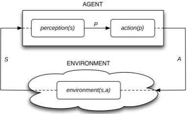
The block diagram of figure 1 shows how the agent works. The Perception block records the changes in the state of the environment. The Action block computes the actions to be taken in order to change the environment. The agent environment changes based on the actions applied by the agent, as well as actions by other agents, and it may be dynamic in that it may change by itself.
An agent can also have an internal state as a deci-sion mechanism for the actions to undertake. An agent with perception and internal state capabilities has more computational power than an agent without them and its computational power is now comparable with that of the Belief-Desired-Intention architecture as described by Wooldridge in [7].
Definition 1: (Purely reactive agents with no internal state) The environment consists of a set of states S =
{s1, s2,· · ·}. The agent can undertake a set of actions A = {a1, a2,· · ·} and perceive a set of percepts P = {p1, p2,· · ·}. For a purely reactive agent, the behavior of the agent can be represented as the function
action:P 7→A (1)
for the action block (refer to figure 1), and the function
perception:S7→P (2)
for the perception block. The deterministic behavior of an environment can be represented by the function
environment:S×A7→S. (3)
perception(s) action(p)
environment(s,a) P
A S
AGENT
ENVIRONMENT
Fig. 1. Agent abstract architecture block diagram.
The perception part has to do with the way the agent senses the environment, which is called a percept. The perception function maps the environment state into a percept.
Having the perception mechanism provides a complete and more general characterization of the agent’s abstract architecture by separating the sensory capabilities (per-ception) from the decision making capabilities (action). It is intended to represent the agent’s capability of sensing the environment. Suppose that the agent will take the same actions for environmental states s1 and s2. This means that both states have the same percept:perception(s1) = perception(s2) = p1, and then the action function will execute the same action as if it depends on the percepts instead of the environmental state.
Agents can also be defined with an internal state and the actions that the agents undertake depend on the internal state only. Figure 2 presents a block diagram of the complete abstract architecture. From this we can see that the capabilities of the abstract architecture previously pre-sented are now enhanced in the complete definition, but the essential perception/action paradigm is still consistent. An intelligent agent with internal state will react to the changes in its internal state instead of reacting directly to the changes in the environment. The internal state will then change based on changes in the environment as processed by the perception mechanism.
Definition 2: (Purely reactive agents with internal state) Let a discrete set I={i1, i2,· · ·}be the set of all internal states, and S andP be the set of environmental states and percepts respectively as described in defini-tion 1. Then the action(·) function will be defined as action:I7→AwhereAis the set of actions as described before. Since the agent’s actions are now dictated by the evolution of the internal state and not that of the environment, an additional function is needed to describe that evolution as a function of the percepts and the current state; that function is defined asnew state:I×P 7→I. An execution loop is defined for the complete abstract architecture in [7].
B. Communication and interaction
Environment Agent A
perception
new_state
action
Internal State
Fig. 2. Complete definition of the intelligent agent abstract architecture.
meaning in a certain context. A communication protocol defines a language for the exchange and understanding of messages between the agents [3], [5], [7]. Interaction in multi-agent systems is the way conversations take place among agents, which is provided by a structure for the exchange of messages. Such conversation is the passing of multiple messages among agents both ways. Interaction deals with a higher level of abstraction than communication. It defines if the agents will cooperate to execute tasks, or will compete for resources, or if they will engage in negotiations in order to fulfill their individual goals in the case of self-interested agents.
The interaction mechanism in multi-agent systems is the structure of the conversations that can take place among agents, and it is intended to provide social be-havior which is essential to achieve system level goals [23]. Several issues related to interaction are present in the design of a multi-agent system. The interactions depend on the problem decomposition. As a result, there will be a need to try different types of interactions from the ones currently described in the literature or develop a new methodology for the specific problem [8], [23]. It is also not clear how to ensure coherence. The rule of thumb is to exploit positive interactions and avoid negative interactions but there is no clear methodology to identify conflicts nor direct how to solve them [8], [23]. It is also not clear how to coordinate the agents and how to make the agents reason about such coordination [8].
III. INTRODUCTION TOPETRI NETS
Petri nets are a graphical and mathematical modeling tool used to describe and analyze different kinds of real systems. Petri nets were first introduced by Carl Adam Petri in 1962 in Germany [15], and evolved as a suitable tool for the study of systems that are concurrent, asynchronous, distributed, parallel and/or stochastic. A multi-agent system is a kind of DEDS that is concurrent, asynchronous, stochastic and distributed. From the DEDS point of view, multi-agent systems lack analysis and design methodologies. Petri net methods are used in this study to develop analytical methodologies for multi-agent systems.
A. Petri nets definition
Definition 3: The following is the formal definition of aPetri net[14], [15], [29], [30]. A Petri net is a five-tuple
(P, T, A, W, M0) (4)
where:
P is a finite set of places
T is a finite set oftransitions
A⊆(P×T)∪(T ×P)is a set of arcs
W :A7→ {1,2,3, . . .} is aweightfunction M0:P 7→Z+ is the initialmarking
The meanings of places and transitions in Petri nets depend directly on the modeling approach. When model-ing, several interpretations can be assigned to places and transitions. For a DEDS a transition is regarded as an event and the places are interpreted as a condition for an event to occur.
Places, transitions and arcs: Places are represented with circles and transitions are represented with bars. The arcs are directed from places to transitions or from transitions to places. The places containtokensthat travel through the net depending on the firing of a transition. A place p is said to be an input place to a transition t if an arc is directed from ptot. Similarly an output place of t is any place in the net with an incoming arc from transition t.
Transition firing: A transition can fire only if it is enabled. For a transition t to be enabled, all the input places of t must contain at least one token1. When a transition is fired, a token is removed from each input place, and one token is added to each output place. In this way the tokenstravel through the net depending on the transitions fired.
Definition 4: (Marking) The marking mi of a place
pi ∈ P is a non-negative quantity representing the
number of tokens in the place at a given state of the Petri net. The marking of the Petri net is defined as the function M : P 7→ Z+ that maps the set of places to the set of non-negative integers. It is also defined as a vector Mj = (m1, m2,· · ·, m|P|) were mi = M(pi),
which represents the jth state of the net. M
j contains
the marking of all the places and the initial marking is denoted by M0.
The marking of the Petri net represents the state of the net. As described above, the transitions change the state of the Petri net in the same way an event changes the state of a DEDS.
Definition 5: (Reachability graph) The reachability graph has the marking of the Petri net (or state of the Petri net) as a node. An arc of the graph joiningMi with
Mj represents the transition when firing takes the Petri
net from the marking (state)Mi to the markingMj.
B. Properties
This section covers some of the most important prop-ertiesof Petri nets such asReachability, Liveness, Bound-edness andReversibility. These are properties that could be applied to multi-agent systems models. Examples of these properties are boundedness and liveness since they are related to deadlock avoidance in DEDS. Other properties are going to be relevant to multi-agent systems particularly to the communication, interaction, and single agent architectures. The analysis methods developed in this research will focus on the following properties.
Definition 6: (Reachability) A markingMj is said to
be reachable from markingMi if there exists a sequence
of transitions that takes the Petri net from state Mi to
Mj . The set of all possible markings that are reachable
from M0 is called the reachability set and is defined by R(M0).
The concept of reachability is essential for the study of the dynamic properties of a Petri net [15], [28].
Definition 7: (Liveness) A Petri net is said to be live for a marking M0 if for any marking in R(M0) it is possible to fire a transition.
The liveness property guaranties the absence of dead-lock in a Petri net. This property can also be observed from the reachability graph. If the reachability graph contains an absorbent state, then the Petri net is not live at that state and it is said to have a deadlock [15], [28].
Definition 8: (Boundedness) A Petri net is said to be bounded or k-bounded if the number of tokens in each place does not exceed a finite numberkfor any marking in R(M0). Furthermore, a Petri net is structurally bounded if it is bounded for any finite initial markingM0. A Petri net is said to be safe if it is 1-bounded[15].
Definition 9: (Reversibility)A Petri net isreversible, if for any marking inR(M0),M0 is reachable. This means that the Petri net can always return to the initial marking M0 [15], [28].
C. Structural analysis
The liveness and boundedness of the net will be assessed by using P-invariants and T-invariants. These invariants are obtained from the incidence matrix of the net and they are used to assess the overall liveness and boundedness of the net.
Definition 10: (Incidence matrix)Leta+ij=w(i, j)be the weight of the arc that goes from transitionti to place
pj anda−ij =w(j, i)be the weight of the arc from place
pj to transition ti. The incidence matrixAof a Petri net
has |T| number of rows and |P| number of columns. It is defined asA= [aij] whereaij =a+ij−a
−
ij.
Definition 11: (Net-invariants)LetAbe the incidence matrix. A P-invariant is a vector that satisfies the equation
Ax= 0 (5)
and a T-invariant is a vector that satisfies the equation
ATy= 0. (6)
1) Boundedness assessment: A Petri net model is covered by P-invariants if and only if, for each place s in the net, there exists a positive P-invariant xsuch that x(s)>0. Furthermore, a Petri net is structurally bounded if it is covered by P-invariants and the initial markingM0 is finite.
2) Liveness assessment: A Petri net model is covered by T-invariants if and only if, for each transition tin the net, there exists a positive T-invariantysuch thaty(t)>0. Furthermore, a Petri net that is finite is live and bounded if it is covered by T-invariants. This is a necessary condition but not sufficient.
IV. RESULTS IN MODELING MULTI-AGENT SYSTEMS USINGPETRI NETS
A simple multi-agent system is presented and studied in this section. The multi-agent system is modeled using the abstract architecture representation presented in section II-A. In addition, the multi-agent system is modeled using a Petri net with the intention of carrying out a structural analysis of the multi-agent system as a discrete-event system, that is, focusing on thelivenessandboundedness, as they relate to the absence of deadlock in the system.
The multi-agent system presented here is loosely based on the behavior of ants as they move food from one place to another. The system consists of two ants, and each one will be modeled as an intelligent agent. They move objects from one place to another which will be the environment of the agents. The system under consideration can be viewed in two different ways: a) the system consists of two “physical” agents and the abstract architecture and Petri nets are used to model their behavior; b) the abstract architecture and Petri nets are used to model, analyze and design the reasoning/control of the two agents so they could perform their intended tasks in such an environment.
environmental states for each agent. A Petri net modelN3 is also presented to help demonstrate why the modeling approach (selection of places and transitions and detail level) is important to ensure that the key properties are captured by the Petri net model. It supports the theory that the abstract architecture can be used as an intermediate step to obtain a Petri net model.
A. Description of the multi-agent system
This section presents a description of a simple multi-agent system consisting of two physical multi-agents that work together at a task. This system will be used throughout this section to illustrate how the Petri net and abstract architecture models can be applied to multi-agent systems. This system consists of two agents referred to asagent Aandagent B. They move objects from one end of a path to the other. Figure 3 shows 4 scenarios in the operation of the system. Both agents are capable of moving objects and agent A moves faster than agent B. The objective of agent A is to go to the end of the path, pick an object, and return to the start of the path (figure 3a). Since it is faster than agent B it reaches the objects first (figure 3b). At the time they intersect in the path, agent A gives its object to agent B and returns to the end of the path to pick another object (figures 3c and 3d). On the other hand, the objective of agent B is to go in the direction of the end of the path, intersect with agent A and get its object. Once the agent has an object, it returns to the start of the path, places the object down and starts all over again.
B A
Move objects a)
B
A
Move objects b)
B A
Move objects c)
B A
Move objects d)
Fig. 3. Multi-agent system for modeling and analysis.
The meta level environment of the system consists of a single path with a set of objects on one side and no objects on the other side. The amount of objects at the end of the path can be considered finite or infinite and both cases will be considered in the following sections (see table I).
There is indirect interaction between the agents via changes in their environments. The exchange of the object between the agents should be regarded as a result of a change in the environment of both agents. The two agents are regarded aspurely reactive, which implies they do not have a record of history and they do not have an internal state. The decisions they make are about which actions to undertake and those decisions are directly influenced by the location of the agent in the path and whether the agent
has an object or not. It should be noted also, that the goal of the overall multi-agent system is a little different from the goal of each specific agent.
TABLE I
DESCRIPTION OF MODELS APPLIED TO THE MULTI-AGENT SYSTEM.
Case Description Petri net Abstract architecture
1 Infinite number of objects N1 M1
to move.
2 Finite number of objects N2 –
to move.
3 Finite number of objects N3 M3
to move. Added capabilities to agents to handle finite number of objects.
B. Case 1: Petri net and abstract architecture models
The multi-agent system described in the previous sec-tions is studied here considering there is an infinite number of objects at the end of the path that are going to be moved to the start of the path by the agents. A Petri net model (N1) of the system is presented and analyzed in order to check that the system is bounded and deadlock free. In addition, an abstract architecture model (M1) is presented for both agents. The objective is to show how a multi-agent system can be modeled using the abstract architecture, as well as the Petri net methodologies.
1) Modeling as a discrete-event system using Petri nets: This section presents a Petri net model of the multi-agent system described in section IV-A. It assumes that the number of objects available at the end of the path is in-finite. This implies that the system should operate without interruption based on the described agents’ capabilities. The multi-agent system is considered as a discrete-event system and the liveness and boundedness properties are analyzed to check if the system is deadlock free. The purpose of this model is to show the ability of Petri net methodologies to model multi-agent systems including the agents interaction.
Several interpretations can be assigned to places and transitions. In the Petri net model presented in this sec-tion places model the activity that a particular agent is performing. Having a token in a place that represents a specific activity means that the agent is currently perform-ing such activity. The transitions model the termination of an activity of a particular agent. Firing a transition indicates that the agent finished performing the activity indicated by the input place and will start performing the activity of the output place.
pA1
pA2
pA3
px
pB1
pB2
pB3 t1
t2
t3
t5
t4
t6
Fig. 4. Petri net modelN1for system with infinite number of objects.
TABLE II
PLACES DESCRIPTION FORN1.
Places (P) Description
pA1 Agent A going to the end of the path to pick object
pA2 Agent A is at the end of the path loading an object
pA3 Agent A is going to start of the path to intersect
with agent B
pB1 Agent B going to the end of the path to intersect
with object A
pB2 Agent B going to the start of the path to leave object
pB3 Agent B unloading object at the start of the path
px Both agents are exchanging the object
2) Analysis of the reachability graph: At this point we are concerned with the net being bounded and live. An assessment of these properties based on the initial marking of the net can be performed by analyzing the reachability tree of N1, using M0 as the root node as shown in figure 5. A reachability tree is a graph representation of the markings of a net. Each node in the tree represents a marking and the edges represent a transition firing [15]. The resulting tree is small enough to be analyzed by inspection and it can be concluded that: a) the reachability set R(M0) is finite, b) the number of tokens of every place in all markings is bounded (1−bounded), and c) there are no dead transitions (all transitions can fire). As a result, it can be concluded that the net is bounded.
By looking at the reachability graph ofN1 with initial markingM0presented in figure 6, it can be seen that there is always an active transition regardless of the state of the net, and all the transitions ofT are included in the graph.
M0=[1 0 0 0 1 0 0]
M1=[0 1 0 0 1 0 0]
M2=[0 0 1 0 1 0 0]
M3=[0 0 0 1 0 0 0]
M4=[1 0 0 0 0 1 0]
M8=[0 1 0 0 0 1 0] t1
t2
t3
t4
M5=[1 0 0 0 0 0 1] t6
t1
M0: "old" t5
M6=[0 1 0 0 0 0 1] t1
M7=[0 0 1 0 0 0 1] t2
M1: "old" t5
M2: "old" t6 M6: "old"
t6
M9=[0 0 1 0 0 1 0] t2
t6
M7: "old"
Fig. 5. Reachability tree ofN1.
From this it can be concluded that the Petri net model of the multi-agent system is bounded and live. This implies that the interaction between the agents does not fall into deadlocks.
M0 M1 M2 M3 M4 M5
M8
M6
M7 M9
t1 t2 t3 t4
t1
t2
t6
t6 t1 t6
t2 t5
t6
t5
Fig. 6. Reachability graph forN1.
For models with a large number of places and transi-tions, the reachability graph construction is not practical without the use of computer tools to automate the reach-ability graph generation and the assessment of properties. Under this scenario, it is preferable to use the algebraic network representation (incidence matrix) and invariance theorems to assess the structural net properties.
of the incidence matrix (invariant analysis) as described in section III-C. The incidence matrix is defined as A = [aij], where aij =a+ij −a
−
ij, a
+
ij = w(i, j) is the
weight of the arc from ti to pj, and a−ij =w(j, i)is the
weight of the arc frompj toti. LetA1 be the incidence matrix of N1. The order of the places in the matrix is P = {pA1, pA2, pA3, px, pB1, pB2, pB3} (columns), and the order of the transitions is T = {t1, t2, t3, t4, t5, t6} (rows).
A=
−1 1 0 0 0 0 0
0 −1 1 0 0 0 0
0 0 −1 1 −1 0 0
1 0 0 −1 0 1 0
0 0 0 0 1 0 −1
0 0 0 0 0 −1 1
(7)
A P-invariant is a vector that satisfies the equation Ax = 0, and a T-invariant is a vector that satisfies the equation ATy = 0. The following invariants were ob-tained from the incidence matrixA1. The T-invarianty1=
[1,1,1,1,1,1]T, the P-invariantsx1= [1,1,1,1,0,0,0]T, andx2= [−1,−1,−1,0,1,1,1]T.
A net is said to be covered by P-invariants if and only if, for each place pin the net, there exists a positive P-invariantxsuch thatx(p)>0. The netN1 is covered by P-invariants since there is a positive element either onx1 orx2for every place, e.g.,x1(pB1) = 0butx2(pB1) = 1. In addition, a net is covered by T-invariants if and only if, for each transitiont in the net, there exists a positive T-invariant y such thaty(t)>0. N1 is also covered by T-invariants.
A Petri net is structurally bounded if it is covered by P-invariants and the initial marking M0 is finite. Furthermore, a net is live and bounded if it is covered by T-invariants; this is a necessary condition only. The Petri net N1 is covered by T-invariants and P-invariants. Since the initial marking is finite, we can conclude that the Petri net is bounded and that the necessary condition for liveness is met.
Discussion: A marked graph is a subclass of Petri nets where each place has exactly one incoming arc and exactly one outgoing arc [15] [30]. There is a theorem that states that every marked graph is live and also bounded if the initial marking is bounded [15]. The net N1 is a marked graph andM0is bounded, therefore the net is live and bounded.
4) Abstract architecture model: The abstract architec-ture of intelligent agents presented in section II-A is used here to model the multi-agent system with an infinite number of objects present. Agents will be considered to be purely reactive where the environment consists of a set of states S = {s1, s2,· · ·}, the agent can undertake a set of actions A = {a1, a2,· · ·}, and perceive a set of percepts P = {p1, p2,· · ·}. For a purely reactive agent, the behavior of the agent can be represented as the function action : P 7→ A and perception : S 7→ P.
The deterministic behavior of an environment can be represented by the functionenvironment:S×A7→S. Let M1 be the multi-agent system with agents A and B modeled with the abstract architecture. The model presented below assumes thatP =S for both agents, as a result action:S 7→A.
Abstract model for agent A: Agent A can undertake a set of actions AA, its environment is defined by SA
and the functionactionAdefines the actions to undertake
based on the changes in the environment. The following tables describe the abstract model for this agent, the en-vironmental states and actions descriptions are presented in tables III and IV respectively; equation 8 defines the action function.
TABLE III
DESCRIPTION OF STATES FOR AGENTAOFM1.
States (SA) Description
s1 Agent has object
s2 Agent has no object and it is not at the end
s3 Agent has no object and it is at the end
TABLE IV
DESCRIPTION OF ACTIONS FOR AGENTAOFM1.
Actions (AA) Description
a1 Walk to the end
a2 Pick an object
a3 Walk to start
actionA(s) =
a1 ifs=s2 a2 ifs=s3 a3 ifs=s1
(8)
It should be noted that agent A has no actions for the exchange of an object at the intersection with agent B. Agent B is assumed to take over the object from agent A, thus changing the environment of agent A and incurring an indirect interaction.
Abstract model for agent B:Agent B can undertake a set of actions AB, its environment is defined by SB and the
function actionB defines the actions to undertake based
on the changes in the environment. The environmental states and actions descriptions are presented in tables V and VI respectively; equation 9 defines the action function. Agent B is assumed to take over the object from agent A when they intersect. This action is reflected in AB and functionactionB.
TABLE V
DESCRIPTION OF STATES FOR AGENTBOFM1.
State (SB) Description
s1 Agent has no object
s2 Agent has object and it is not at the start
s3 Agent has object and it is at the start
TABLE VI
DESCRIPTION OF ACTIONS FOR AGENTBOFM1.
Action (AB) Description
a1 Walk to the end
a2 Take over object from agent A
a3 Walk to start
a4 Put object down at start
actionB(s) =
a1 ifs=s1 a2 ifs=s4 a3 ifs=s2 a4 ifs=s3
(9)
5) Discussion: The analysis performed in this sec-tion (case 1) shows that the multi-agent system under consideration has appropriate structural properties. This system will not go into a deadlock and will work correctly under the current modeling assumptions. Assumptions with respect to the agents’ behavior may not hold if the assumptions in the agents environment change. The strongest assumption in this scenario case 1 (for abstract model M1 and Petri net model N1) is the fact that the number of objects to move is infinite. If this is changed to a finite number of objects, the current agent behavior may not work for the overall system objective; in fact, the multi-agent system will deadlock.
When analyzing the abstract model M1 when this assumption does not apply, it can be seen that eventually, agent A will reach state s3 and no object will be there to be picked. Then, action a3 will have no effect and will not change the state of the local environment. In the case of agent B, it will eventually remain at state s4and action a2 will not be executed as expected. In the case of the Petri net modelM1,t2 will never fire even if it is active because the activity modeled by place pA2 cannot be concluded without objects to pick. This model fails and no longer represents the dynamics of the real system.
C. Case 2: Petri net model
The multi-agent system described in section IV-A is studied here considering now that there is a finite number of objects at the end of the path. Since the agents do not have the capability to handle a lack of objects to transport, it is expected that the system falls into deadlock. A Petri net model (N2) is presented and analyzed in order to check that the system falls into deadlock.
1) Petri net model and analysis: Let N2 =
(P, T, A, W, M0) be the Petri net presented in figure 7 that models the multi-agent system under consideration. It is based on netN1presented in the previous section to model an infinite number of objects. An additional place was added to the previous model in order to include a representation of the finite number of objects to be moved from the end to the start of the path. This additional place will serve as abuffer place, and should be linked in a way to the action taken by agent A when picking the object at the end of the path. The buffer placepb was added to
model the finite number of objects. Transition t2 is now active when there is a token in place pA2 (agent A is at the end of the path loading an object) and there is at least one token in place pb (there is at least one object at the
end of the path). From inspection of the Petri net it can be seen that eventually the net execution will reach a state with no enabled transitions. Consider the instance where M(pb) = 0(no more objects available at the end of the path) and M(pA2) = 1. Transitiont2can not be enabled anymore becausepbworks as a source of tokens and have
no incoming arcs from other transitions, therefore the net is not live.
pA1
pA2
pA3
px
pB1
pB2
pB3
t1
t2
t3
t5
t4
t6
pb
k tokens
Fig. 7. Petri net modelN2for system with finite number of objects.
The description of places P =
{pA1, pA2, pA3, px, pB1, pB2, pB3, pb} for N2 is the same as that of N1 presented in table II, plus the buffer place pb described above. The transitions
T = {t1, t2, t3, t4, t5, t6} have the same interpretation and the initial marking M0 = [1,0,0,0,1,0,0, k] where k is a positive integer denoting the number of objects in the path. The weights of the arcs are all one as inN1.
The liveness and boundedness properties can be verified by inspection of the reachability graph or by analysis of the incidence matrix which is the approach presented for this case. The reachability graph will be large even for smallkand it will be impractical to build by hand, but it is easy to visualize that it will contain at least one node with no outgoing arc, e.g., Mi = [0,1,0,0,1,0,0,0] (where
M0. A similar reasoning can be used to see that there is no unbounded place in R(M0). At any execution point of the net, the largest marking is that of place pb, with
M(pb) =k at the initial marking. As a result, any place of the network will have a marking less than or equal to k, hence the net is bounded.
The structural analysis can be carried out in this case. Let A2 be the incidence matrix of the model. The order of the places in the matrix is now P =
{pA1, pA2, pA3, px, pB1, pB2, pB3, pb}, and for transitions
it is T ={t1, t2, t3, t4, t5, t6}. The incidence matrix has no T-invariants sinceA0y= 0has only the trivial solution y = 0. The P-invariants are x1 = [1,1,1,1,0,0,0,0]T and x2 = [−1,−1,−1,0,1,1,1,0]T. Therefore, the net is neither covered by T-invariants nor P-invariants.
A2=
−1 1 0 0 0 0 0 0
0 −1 1 0 0 0 0 −1
0 0 −1 1 −1 0 0 0
1 0 0 −1 0 1 0 0
0 0 0 0 1 0 −1 0
0 0 0 0 0 −1 1 0
(10) Since the net is not covered by P-invariants we cannot use this method to assess boundedness. Similarly, we cannot assess liveness directly, if it is assumed that the net is bounded, and taking into account that M0 is finite, it can be concluded that the net is not live due to the fact that it is not covered by T-invariants and the necessary condition is not met.
2) Discussion: This model also shows how the analy-sis by visual inspection of the reachability graph quickly becomes cumbersome indicating the need for computa-tional tools even for small systems. On the other hand, it also shows that the structural analysis theorems are not always useful and other techniques are required. Another way to perform the analysis will be to reduce the Petri net model into one with a smaller number of places and transitions that preserves the liveness and boundedness properties. The smaller model can then be analyzed by means of the reachability graph.
D. Case 3: Abstract and Petri net models
The abstract model M1 presented in case 1 (section IV-B) can be modified to allow the system to behave properly when there are a finite number of objects to be moved. In Case 1 the Petri net model assumed an infinite number of parts, as a result the system never deadlocks. On the other hand, Case 2 considered a finite number of parts and the system deadlocked. The abstract model for case 1 did not consider the fact that there could be finite resources. Basically, we can increase the number of environmental states S of the agents A and B, so they will now allow the fact that there might not be any object to pick up at the end of the path.
There should be a new state for each of the agents of the multi-agent system and a set of actions to perform when there are no more objects at the end of the path.
The state and action for each of the agents can be defined independently. Lets consider agent A to remain at the end of the line until more objects are available. In order to make use of the previous strategy now agent B must return to the start of the path when there is no part to take over in the intersection with agent A. Note that in the case of no parts left, the intersection will happen at the end of the path.
1) Abstract model for Case 3: LetM3be a multi-agent system with agents A and B modeled with the abstract architecture and let P =S (action :S 7→A). Agent A can undertake a set of actionsAA, its environmental states
are SA, and actionA defines the actions to undertake
based on the changes in the environment. In addition, Agent B can undertake actions AB, its environment is
defined by SB, and the action functionactionB. a) Abstract model for agent A:: The following tables describe the upgraded abstract model for agent A. There is one additional action and an additional state. Tables VII and VIII show the states and actions descriptions respectively, actionA is presented in equation 11.
TABLE VII
DESCRIPTION OF STATES FOR AGENTAOFM3.
State (SA) Description
s1 Agent has object.
s2 Agent has no object and it is not at the end.
s31 Agent has no object, it is at the end of the path
and there are available objects.
s32 Agent has no object, it is at the end of the path
and there are no available objects.
TABLE VIII
DESCRIPTION OF ACTIONS FOR AGENTAOFM3.
Actions (AA) Description
a1 Walk to the end
a2 Pick an object
a3 Walk to start
a4 Wait for more objects
action(s) =
a1 ifs=s2 a2 ifs=s31 a3 ifs=s1 a4 ifs=s32
(11)
b) Abstract model for agent B:: Agent B is assumed to take over the object from agent A when they intersect. The additional environment state allows agent B to behave properly when it is at the intersection with agent A and there is no object to take over. Table IX presents the description of the environmental states, table X is the description of the actions the agent can undertake, and equation 12 is the function actionB.
action(s) =
a1 ifs=s1 or s=s42 a2 ifs=s41
a3 ifs=s2 a4 ifs=s3 a5 ifs=s5
TABLE IX
DESCRIPTIONS OF STATES FOR AGENTBOFM3.
State (SB) Description
s1 Agent has no object
s2 Agent has object and it is not at the start
s3 Agent has object and it is at the start
s41 Agent is at the intersection and there is a part
s42 Agent is at the intersection and there is no part
s5 Agent is at the end of the path (no objects available)
TABLE X
DESCRIPTION OF ACTIONS FOR AGENTBOFM3.
Actions (AB) Description
a1 Walk to the end
a2 Take over object from agent A
a3 Walk to start
a4 Put object down at start
a5 Wait
2) Petri net model: The multi-agent systems presented in this section will work properly when there are no more objects at the end of the path. The added capabilities make the agents wait at the end of the path until more objects are available.
Let N3 = (P, T, A, W, M0) be the Petri net that models the multi-agent system under consideration. Fig-ure 8 shows the Petri net model of the system and table XI presents the description of the places P =
{pA1, pA2, pA3, px, pB1, pB2, pB3, pb, pint}. The
transi-tions areT={t1, t2, t3, t4, t5, t6, t7}and the initial mark-ing M0 = [1,0,0,0, 1,0,0, k,0]. The new capabilities consist only of waiting for more objects to be available in order to be able to move. This capability is already modeled since agent A will remain in placeP A2(waiting for more objects to be available). In the case of agent B, this will be reflected in place Pint but in the original
model N2 (figure 7) place P B2 could also model this capability.
TABLE XI
PLACES DESCRIPTION FORN3.
Place Description
P A1 Agent A going to the end of the path to pick object
P A2 Agent A is at the end of the path loading an object or
waiting
P A3 Agent A is going to start of the path to intersect with
agent B
P B1 Agent B going to the end of the path to intersect with
agent A
P B2 Agent B going to the start of the path to leave object
P B3 Agent B unloading object at the start of the path
Px Both agents are exchanging the object
Pint Agent B is at an intersection at the end of the line waiting for more objects
3) Discussion: The modeling approach used previ-ously models agent activities as places. Having a token in a place means that an agent is executing the activity indicated by the place. The modeling approach is now important because previous results show that there is no
pA1
pA2
pA3
px
pB1
pB2
pB3
t1
t2
t3
t5
t4
t6
pb
k tokens
t7
pint
Fig. 8. Petri net model ofN3.
uniqueness in the Petri net models obtained. The objective of modeling the multi-agent system as a discrete-event system is to analyze structural properties, and use those results to infer something about the behavior of the multi-agent system and its interaction protocol.
V. MODELING OFMULTI-AGENTSYSTEMS WITH
INDIRECTINTERACTION
The methodology presented here consists of defining a simple multi-agent system based on the abstract architec-ture for intelligent agents (M4). The abstract architecture is modeled as a discrete-event system using Petri nets (N4) and structural and reachability analysis provides an assessment of the interaction properties.
The purpose of this work consists of the definition of an abstract architecture for multi-agent systems with indirect interaction, analogous to the abstract architecture for intelligent agents. The proposed architecture allows the description of agent-to-agent interactions via changes in the environment and serves as an initial description of the discrete-event dynamics of the multi-agent system. In addition, this work presents an algorithm (algorithms 5.1 and 5.2) to obtain a Petri net model of a multi-agent system by making use of the multi-agent system’s abstract architecture. Finally, a methodology to ensure that the multi-agent system is deadlock free is presented; it is based on the analysis of the properties of the Petri net model.
another agent’s environment triggering a reaction. The indirect interaction occurs in the cases when two or more agents share a subset of the environment. It should be noted that the overall multi-agent system acts over a macro level environment. An agent that is part of the multi-agent system has its own environment that is somehow related to the macro level environment of the multi-agent system. This macro level environment of the multi-agent system is referred to in the literature as being an open environment [8]. A complex problem will provide an open environment, which is dynamic, has components that are unknown in advance, its structure changes over time and might be heterogeneous in its implementation [8]. By focusing on the interactions among agents as described above, it is natural to regard a multi-agent system as a discrete-event system.
A. Petri net models from the abstract architecture
The artificial intelligence research considers three dif-ferent paradigms for intelligent agents: a) reactive and b) deliberative; and c) hybrids between them. The abstract architecture models how an agent behaves with respect to changes in its environment. Here, an agent has its own environment and this environment is defined by the nature of the agent. The goals, objectives and the general purpose of the agent define its environment. This abstract architecture is based on the reactive paradigm of perception and action. A purely reactive agent has a perception of the environment and it is used in the decision mechanism that provides an action in the agent. A reactive agent can also have an internal state as a decision mechanism for the actions to be undertaken. An agent with perception and internal state capabilities has more computational power than an agent without them and its computational power is now comparable with that of the Belief-Desired-Intention architecture as described in [7].
Abstract model for purely reactive agents:In a purely reactive agent, the perception part records the changes in the state of the environment. The action part computes the actions to be taken in order to react to changes in the environment. The agent environment changes based on the actions applied by the agent, as well as actions by other agents, and it may be dynamic in that it may change by itself.
The environment consists of a set of states S =
{s1, s2,· · ·}. The agent can undertake a set of actions A = {a1, a2,· · ·} and perceive a set of percepts P = {p1, p2,· · ·}. For a purely reactive agent, the behavior of the agent can be represented as the functionaction:P 7→ A and perception:S 7→P. The deterministic behavior of an environment can be represented by the function environment : S×A 7→ S. A detailed explanation of the abstract architecture was presented in section II-A.
Petri net modeling of multi-agent systems:A Petri net is defined as a five-tuple(P, T, A, W, M0)where:P is a finite set of places,T is a finite set of transitions, A⊆
(P×T)∪(T×P)is a set ofarcs,W :A7→ {1,2,3, . . .}
is a weight function, and M0 : P 7→ Z|
P|
+ is the initial marking.
1) Obtaining Petri net models from the abstract ar-chitecture: Places model the environmental state of the agent. Having a token in a place representing state si
means that the agent is currently in such a state. Transi-tions model the actions of an agent. The environmental state is changed by actions so, for the Petri net model having tokens move from one place to another by firing transitions, this agrees with the execution process of the abstract architecture.
Algorithm 5.1: (Petri net sub model for agenti)LetSi
be the set of environmental states of agenti, andsij ∈Si
be the jth environmental state of agent i. Similarly, let Ai be the set of actions of agenti, and aik∈Ai be the
kthaction of agenti.
1) Add a place for each element of the environment Si and label each place using notation Pij for sij.
2) Add a transition for each action in Ai and label
each transition using notationTik foraik.
3) For each instance of the function environment :
Si×Ai 7→Si say sij×aik 7→sil: a) add an arc
leaving from placePij and ending in transitionTik;
b) add an arc leaving from transitionTikand ending
in placePil; c) add a weight of 1 to each arc.
If an arc from transition Tik to place Pil already
exists, add a new transition and label itTik0 ; perform this step usingTik0 instead ofTik.
4) Add a token in the place representing the initial state of the environment.
Algorithm 5.2: (Petri net model of the multi-agent sys-tem) The Petri net sub-models of each of the individual agents in the system should be joined based on their indirect interactions. In general, this indirect interaction will be in such a way that an agent iaction will change an environment state of agent j. This communication act can be regarded as a regular action in the construction of the complete model. There will be arcs added from the places modeling the environmental states of agentjto the transition modeling the communication in agent i.
2) Analysis of the Petri net model: Inspection of the reachability graph of the Petri net model can indicate if the model is live and bounded. On the other hand, liveness and boundedness properties can also be assessed using invariant analysis [30].
B. Case 4: Multi-agent system modeling and analysis
via changes in their environments. The interchange of the object between the agents should be regarded as a result of a change in the environment of both agents. It should be noted that there is no way to avoid the interaction since it is assumed that the agents meet (see figure 3c) in the path and they cannot avoid each other. The two agents are regarded as purely reactive, which implies they do not have a record of history and they do not have an internal state.
The objective of agent A is to go to the end of the path, pick an object and return to the start of the path (figure 3a). Since it is faster than agent B, at the time they intersect in the path, agent A gives its object to agent B and returns to the end of the path to pick another object. In addition, the objective of agent B is to go in the direction of the end of the path, intersect with agent A and get its object. Once the agent has an object, it returns to the start of the path, places the object down and starts all over again.
The exchange of the object in the intersection of the two agents on the path is only a capability of agent B. As a result, agent A will only react to it but will have no intelligence on that matter. The decisions they make are about which actions to undertake and those decisions are directly influenced by the location of the agent in the path and whether or not the agent has an object.
1) Abstract architecture description: Under normal conditions, agent A will be walking to the end of the path to pick the object to be moved. The object is going to be taken away by the other agent at the intersection. LetM4 be the multi-agent system with agent A and B modeled with the abstract architecture. Agent A has environmental statesSA, a set of actionsAA, an action functionactionA,
and an environment evolution function environmentA.
On the other hand, Agent B has environmental statesSB,
a set of actions AB, an action function actionB, and an
environment evolution function environmentB. Tables
XII and XIII describe the possible environmental states (SA) and the actions (AA) that agent A can undertake.
TABLE XII
ENVIRONMENTAL STATES OF AGENTAOFM4.
State (SA) Description
s1 Agent has object
s2 Agent has no object and it is not at the end
s3 Agent has no object and it is at the end
TABLE XIII ACTIONS FOR AGENTAOFM4.
Actions (AA) Description
a1 Walk to the end
a2 Pick an object
a3 Walk to start
Table XIV presents the mapping of the environment (environmentA) describing how it will be changing as
the agent undertakes actions. It should be noted that
the notion of exchanging the part with agent B at the intersection has not been considered explicitly in the description of theenvironmentA:S×A7→S for agent
A. The agents decision mechanism is described by the actionA function as presented in (13).
TABLE XIV
ENVIRONMENT FUNCTION FOR AGENTAOFM4.
AA SA SA Description
a1 s2 s3 Walking towards the end of the path.
Eventually will reach the end with no object.
a2 s3 s1 Now the agent has an object.
a3 s1 s1 Walking to the start of the path.
Eventually will lose object to agent B.
actionA(s) =
a1 ifs=s2 a2 ifs=s3 a3 ifs=s1
(13)
Agent B will be walking toward the end of the path until it intersects with agent A which is on its way back to the beginning of the path carrying an object. At the intersection point, agent B takes over the object of agent A and proceeds to return to the beginning of the path to drop the object and start the cycle again. The abstract architecture of agent B is presented in Tables XIV and XV, and theactionB(s)function is described in (14).
TABLE XV
ENVIRONMENTAL STATES FOR AGENTBOFM4.
State (SB) Description
s1 Agent has no object
s2 Agent has object and it is not at the start
s3 Agent has no object and it is at the start
s4 Agent is at the intersection with agent A
TABLE XVI ACTIONS FOR AGENTBOFM4.
Actions (AB) Description
a1 Walk to the end
a2 Take over object from agent A
a3 Walk to start
a4 Put object down at start
actionB(s) =
a1 ifs=s1 a2 ifs=s4 a3 ifs=s2 a3 ifs=s3
(14)
The mapping of the environment of agent B
(environmentB) is presented in Table XVII. The
TABLE XVII
ENVIRONMENT FUNCTION FOR AGENTBOFM4.
AB SB SB Description
a1 s1 s4 Will walk toward the end until intersection
with agent A
a2 s4 s2 Object exchange, now it has an object
a3 s2 s3 Will walk towards start until it reaches it
a4 s3 s1 Will drop the object at start
2) Petri net model: The Petri net model of the multi-agent system was obtained following the procedure de-scribed in algorithm 5.1.
Let N4 = (P, T, A, W, M0) be the Petri net model of the complete system with places P = {pA1, pA2, pA3, pB1, pB2, pB3, pB4}, transitions T = {tA1, tA2, tA3, tB1, tB2, tB3, tB4}, and M0 = [0,1,0,1,0,0,0]. Figure 9 shows N4 and the interpretation of places and transitions is presented in Table XVIII. The Petri net sub-models of the individual agents are not presented due to space limitations but they can be observed from the complete model.
Transition tB2 which models an action of agent B, modifies the environmental state of agent A. The Petri net model can now be analyzed to assess the deadlock property in a systematic way.
The tokens in places pA2 andpB1 represent the initial conditions of agent A and B respectively. The tokens travel through the net representing different environment states for the agents as the system executes. The systems execution scenarios presented in figure 3 can be identified in the Petri net model, e.g., scenario d) of figure 3 will be represented in the Petri net model as having a token inpA2 andpB2.
pA3 pA1
pB1
pB4 pB2
pB3
tA1 tA2
tA3 tB1 tB2 tB3 tB4 pA2
Fig. 9. Petri net modelN4.
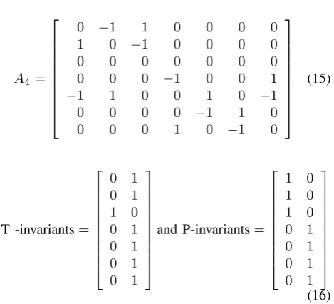
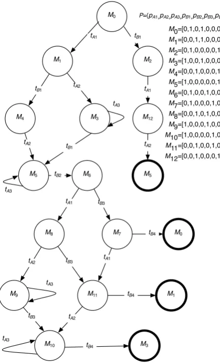
3) Analysis of the Petri net model N4: The Petri net model presented in figure 9 (N4) can now be analyzed to assess the deadlock property of the underlying multi-agent system. The reachability graph of the model is presented in figure 10 and it shows that the net is live and bounded. Therefore, the multi-agent system is deadlock free. Using the incidence matrix (15) of the net and its invariants (16), it is shown that the net is bounded and that the necessary condition for liveness is satisfied; this is a slightly weaker conclusion on “liveness” than when both necessary and sufficient conditions are met.
TABLE XVIII
DESCRIPTION OFPETRI NET MODELN4.
Element Name Description
pA1 A token in this place indicates the
environment is at states1for agent A
pA2 A token in this place indicates the
environment is at states2for agent A
pA3 A token in this place indicates the
environment is at states3for agent A
Places (P) pB1 A token in this place indicates the
environment is at states1for agent B
pB2 A token in this place indicates the
environment is at states2for agent B
pB3 A token in this place indicates the
environment is at states3for agent B
pB4 A token in this place indicates the
environment is at states4for agent B
tA1 Execution of actiona1for agent A
tA2 Execution of actiona2for agent A
tA3 Execution of actiona3for agent A
Transitions (T) tB1 Execution of actiona1for agent B
tB2 Execution of actiona2for agent B
tB3 Execution of actiona3for agent B
tB4 Execution of actiona4for agent B
A4=
0 −1 1 0 0 0 0
1 0 −1 0 0 0 0
0 0 0 0 0 0 0
0 0 0 −1 0 0 1
−1 1 0 0 1 0 −1
0 0 0 0 −1 1 0
0 0 0 1 0 −1 0
(15)
T -invariants= 0 1 0 1 1 0 0 1 0 1 0 1 0 1
and P-invariants= 1 0 1 0 1 0 0 1 0 1 0 1 0 1 (16)
VI. DISCUSSION
M0
M1 M2
M3 M4
M6 M5
M8 M7
M9 M11
M10 M3
M1 M0 M12
M5
tA1 tB1
tB1 tA2
tA2 t
B1
tA3
tA3
tB2
tA1 tB3
tB4
tA2 tB3 tA1
tB4 tA3
tB3 tA2
tB4 tA3
M0=[0,1,0,1,0,0,0] M1=[0,0,1,1,0,0,0] M2=[0,1,0,0,0,0,1] M3=[1,0,0,1,0,0,0] M4=[0,0,1,0,0,0,1] M5=[1,0,0,0,0,0,1] M6=[0,1,0,0,1,0,0] M7=[0,1,0,0,0,1,0] M8=[0,0,1,0,1,0,0] M9=[1,0,0,0,1,0,0] M10=[1,0,0,0,0,1,0] M11=[0,0,1,0,0,1,0] M12=[0,0,1,0,0,0,1] P={pA1,pA2,pA3,pB1,pB2,pB3,pB4}
tA1
tA2
Fig. 10. Reachability graph of Petri net modelN4.
ACKNOWLEDGEMENTS
Portions of this work were supported by NSF grant DMII-0121902.
REFERENCES
[1] M. Greaves, V. Stavridou-Coleman, and R. Laddaga, “Guest ed-itors’ introduction: Dependable agent systems,”IEEE Intelligent Systems, vol. 19, no. 5, pp. 20–23, 2004.
[2] R. Khosla and T. Dillon,Engineering intelligent hybrid multi-agent systems. Kluwer Academic Publishers, 1998.
[3] G. Weiss, Ed., Multiagent systems: a modern approach to dis-tributed artificial intelligence. Cambridge, MA, USA: MIT Press, 1999.
[4] S. S. Heragu, R. J. Graves, B.-I. Kim, and A. St Onge, “Intelligent agent based framework for manufacturing systems control,”IEEE Transactions on Systems, Man and Cybernetics, Part A, vol. 32, no. 5, pp. 560–573, 2002.
[5] N. J. Nilsson,Artificial intelligence: a new synthesis. Morgan Kaufmann Publishers Inc., 1998.
[6] S. J. Russell and P. Norvig, Artificial Intelligence: A Modern Approach. Pearson Education, 2003.
[7] M. J. Wooldridge,Introduction to Multiagent Systems. John Wiley & Sons, Inc., 2001.
[8] K. P. Sycara, “Multiagent systems,”AI Magazine, pp. 79–92, 1998. [9] W. Reisig, Elements of distributed algorithms: modeling and analysis with Petri nets. New York, NY, USA: Springer-Verlag New York, Inc., 1998.
[10] A. A. Desrochers and R. Y. Al-Jaar, Applications of Petri Nets in Manufacturing Systems: Modeling, Control, and Performance Analysis. IEEE Press, 1995.
[11] M. D. Jeng, “A petri net synthesis theory for modeling flexible manufacturing systems,”IEEE Transactions on Systems, Man, and Cybernetics—Part B: Cybernetics, vol. 27, no. 2, pp. 169–183, April 1997.
[12] M. Zhou, F. DiCesare, and A. A. Desrochers, “A hybrid methodol-ogy for synthesis of petri net models for manufacturing systems,”
IEEE Transactions on Robotics and Automation, vol. 8, no. 3, pp. 350–361, 1992.
[13] M. Zhou, K. McDermott, and P. A. Patel, “Petri net synthesis and analysis of a flexible manufacturing system cell,” IEEE Transactions on Systems, Man, and Cybernetics, vol. 23, no. 2, pp. 523–531, March 1993.
[14] T. Agerwala, “Putting petri nets to work,”Computer, vol. 12, no. 2, pp. 85– 94, December 1979.
[15] T. Murata, “Petri nets: Properties, analysis and applications,”
Proceedings of the IEEE, vol. 77, no. 4, pp. 541–580, April 1989. [16] T. Murata, P. C. Nelson, and J. Yim, “A predicate-transition net model for multiple agent planning,”Inf. Sci., vol. 57-58, pp. 361– 384, 1991.
[17] D. Xu, R. Volz, T. Ioerger, and J. Yen, “Modeling and verifying multi-agent behaviors using predicate/transition nets,” in SEKE ’02: Proceedings of the 14th international conference on Software engineering and knowledge engineering. New York, NY, USA: ACM Press, 2002, pp. 193–200.
[18] H. J. Ahn and S. J. Park, “Modeling of a multi-agent system for coordination of supply chains with complexity and uncertainty,” inIntelligent Agents and Multi-Agent Systems, ser. Lecture Notes in Computer Science, J. Lee and M. Barley, Eds., vol. 2891, 6th Pacific Rim International Workshop on Multi-Agents, PRIMA 2003 Seoul, Korea. Springer-Verlag Berlin Heidelberg, November 2003, pp. 13–24.
[19] P. Leit˜ao, A. W. Colombo, and F. Restivo, “An approach to the formal specification of holonic control systems,” inHolonic and Multi-Agent Systems for Manufacturing, ser. Lecture Notes in Computer Science, V. Mar´ık, D. McFarlane, and P. Valckenaers, Eds., vol. 2744, First International Conference on Industrial Ap-plications of Holonic and Multi-Agent Systems, HoloMAS 2003 Prague, Czech Republic, September 1-3, 2003. Springer Berlin / Heidelberg, 2004, pp. 59–70.
[20] F.-S. Hsieh, “Model and control holonic manufacturing systems based on fusion of contract nets and petri nets,” Automatica, vol. 40, no. 1, pp. 51–57, 2004.
[21] M. R. Lyu, X. Chen, and T. Y. Wong, “Design and evaluation of a fault-tolerant mobile-agent system,”Intelligent Systems, vol. 19, no. 5, pp. 32–38, 2004.
[22] A. W. Krings, “Agent survivability: An application for strong andweak chain constrained scheduling,” inHICSS ’04: Proceed-ings of the ProceedProceed-ings of the 37th Annual Hawaii International Conference on System Sciences (HICSS’04) - Track 9. Washing-ton, DC, USA: IEEE Computer Society, 2004, p. 90297.1. [23] S. Bussmann, N. R. Jennings, and M. Wooldridge, Multiagent
Systems for Manufacturing Control. Springer Verlag, 2004. [24] J. M. Vidal. Fundamentals of multiagent systems with netlogo
examples. [Online]. Available: http://www.multiagent.com/fmas [25] S. Kraus,Strategic negotiation in multiagent environments.
Cam-bridge, MA, USA: MIT Press, 2001.
[26] C. Tessier, L. Chaudron, and H.-J. M¨uller, Eds.,Conflicting agents: conflict management in multi-agent systems. Norwell, MA, USA: Kluwer Academic Publishers, 2001.
[27] C. G. Cassandras,Discrete Event Systems, Modeling and Perfor-mance Analysis. Aksen Associates Incorporated, 1993. [28] A. A. Desrochers, “Performance analysis using petri nets,”Journal
of Intelligent and Robotic Systems, vol. 6, no. 1, pp. 65–79, August 1992.
[29] J. L. Peterson, Petri net theory an the modeling of systems. Prentice Hall, 1981.
[30] W. Reisig,Petri nets, An Introduction, ser. EATCS: Monographs on Theoretical Computer Science. Springer-Verlag, 1985, vol. 4. [31] D. Gross and C. M. Harris,Fundamentals of Queuing Theory, ser. Wiley Series in Probability and Statistics. Wiley-Interscience, 1998.
S. degree in Electrical Engineering in 2003, all from Rensselaer Polytechnic Institute, Troy New York; and a B.S. in Cybernetics Engineering in 2001 from CETYS University, M´exico.
Alan Desrochersreceived the B.S.E.E. degree from University of Massachusetts, Lowell, in 1972 and the M.S. and Ph.D. degrees in electrical engineering from Purdue University, West Lafayette, Indiana, in 1973 and 1977, respectively.
During 1974 he was employed in the Guidance and Con-trol Systems Department at the Lockheed Missiles and Space Company, Sunnyvale, California. From 1977-1980, he was an Assistant Professor in the Department of Systems and Com-puter Engineering at Boston University. In 1980, he joined the Electrical and Systems Engineering Department at Rensselaer Polytechnic Institute, Troy, New York. During the 1986-1987 academic year he was a Visiting Scientist in the Laboratory for Information and Decision Systems at MIT, Cambridge, Massachusetts. He is presently a Professor in the Electrical, Computer, and Systems Engineering Department at Rensselaer. He is the author of Modeling and Control of Automated Man-ufacturing Systems, IEEE Computer Society Press,1990, a co-author of Application of Petri Nets in Manufacturing Systems, IEEE Press, 1995 (A. A. Desrochers and R.Y. Al-Jaar), editor of Intelligent Robotic Systems for Space Exploration, Kluwer Academic Publishers, 1992, and co-author of State Variables for Engineers, second edition, John Wiley & Sons, 1998 (P.M. DeRusso, C.M. Close, R. J. Roy, and A.A. Desrochers).
Dr. Desrochers is a past Editor for the IEEE Transactions on Robotics and Automation. In 1987 he was part of a six-faculty member team that received the LEAD award from the Society of Manufacturing Engineers. Since 1995 he has been a Fellow of the IEEE for contributions to manufacturing systems engineering and manufacturing systems education