Vol. 3 Issue 4, April - 2017
www.jmess.org
Instruction: Choice Of Optimum Parameters Of
Technical Systems At The Design Stage
Yu. K. Mashunin
Far Eastern Federal University DVFU
Vladivostok, Russia [email protected]
Abstract—The paper presents a guide: selection of
optimal parameters of technical systems at a design stage. We have presented mathematical model of technical system in the first section. The model is created as a vector problem of mathematical programming. In model criteria (characteristics) are formed in the conditions of definiteness (functional dependence of each characteristic and restrictions on parameters is known) and in the conditions of uncertainty (there is no sufficient information on functional dependence of each characteristic on parameters). We have presented in the second section how the specification (Basic data) for creation of model is formed. Basic data are formed by the designer of technical system (the designer, the client, the customer). In the third section performer (Mashunin Yu. K.) forms mathematical model of technical system. The performer solves a vector problem at equivalent criteria, and reports results to the customer. If necessary the performer solves a vector problem with a priority of this or that criterion and reports results to the customer.
Keywords—Modeling technical systems, Vector optimization, Optimum decision-making, the decision with a criterion priority
I. INTRODUCTION (MATHEMATICAL MODEL OF TECHNICAL SYSTEMS IN THE CONDITIONS OF DEFINITENESS AND UNCERTAINTY IN TOTAL)
The Technique (instruction): "The choice of optimum parameters of technical systems at a design stage" is result of thirty summer researches of the author in the field of vector optimization [1 - 9].
Conditions of definiteness are characterized by that functional dependence of each characteristic and restrictions on parameters of technical system [2 - 8] is known. Conditions of uncertainty are characterized by that there is no sufficient information on functional dependence of each characteristic and restrictions from parameters [4 - 9].
In real life of a condition of definiteness and uncertainty are combined. The model of technical system also has to reflect these conditions. We will
1 Practical problems of simulation of technical systems on this algorithm can be solved with dimensionality of parameters X more than two N>2.
present model of technical system in the conditions of definiteness and uncertainty in total :
Opt F(X) = {max F1(X) = {max fk(X), k =1,K1def }, (1)
max I1(X) {max{fk(Xi, i=1,M)}T, k= unc K1
,
1 }, (2)
min F2(X) = {min fk(X), k =1,K2def }, (3)
min I2(X) {min{fk(Xi, i=1,M)}T, k= unc K2
,
1 }}, (4)
at restrictions xminj xjx
max
j , j =1,N
N
,1
, (5)
where X - a vector of operated variable (design data) equivalent (1); F(X)={ F1(X) F2(X) I1(X), I2(X)} - vector
criterion which everyone a component represents a vector of criteria (characteristics) of technical system (2) which functionally depend on discrete values of a vector of variables X ; F1(X), F2(X) - a set of the max
and min functions respectively; I1(X) и I2(X) set of
matrixes of max and min respectively; K1def, Kdef2
(definiteness), Kunc1 , Kunc2 (uncertainty) the set of criteria of max and min created in the conditions of definiteness and uncertainty;
in (9) fmink fk(X)f max
k , k=1,K – a vector function of
the restrictions imposed on functioning of technical
system xminj xjxmaxj , j =1,N– parametrical restrictions.
II. TERMS OF REFERENCE: "THE CHOICE OF THE
OPTIMAL TECHNICAL PARAMETERS OF THE SYSTEM”
(PERFORMED TECHNICAL SYSTEM DESIGNER)
A. Total
We will consider a task "Numerical modeling of technical system" in which data on some set of functional characteristics (definiteness conditions), discrete values of characteristics (an uncertainty condition) and the restrictions imposed on functioning of technical system are known. The numerical problem of modeling of technical system is considered with equivalent criteria and given priority of criterion.
B. The technical assignment
It is given. The technical system, which functioning is defined by three parameters1X={x
1, x2, x3} – a vector
Vol. 3 Issue 4, April - 2017
www.jmess.org (operated) variables. Basic data for the solution of a
task are fore characteristics (criterion) of F(X)={f1(X),
f2(X), f3(X), f4(X)}, which size of an assessment
depends on a vector of X.
Definiteness conditions. For characteristics of f3(X),
f4(X) functional dependence on parameters X (a
definiteness condition) is known:
f1(X) =50+11.55*x1+3.55*x2+1.0*x3+0.0144*x1*x2
-0*x1*x3+0*x2*x3-0.07*x12-0.07*x22-0*x
2 3 . (6)
Parametrical restrictions:
25x1100, 25x2100, 25x3100. (7)
1) Uncertainty condition. For the second, third and fourth characteristic results of experimental data are known: sizes of parameters and corresponding characteristics. Numerical values of parameters X and characteristics of y2(X), y3(X), y4(X) are presented in
table 1.
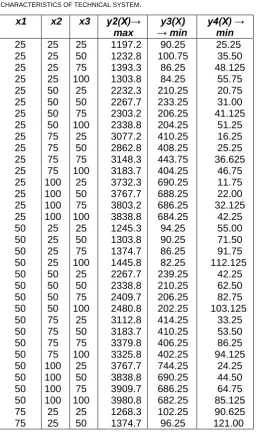
TABLE I. NUMERICAL VALUES OF PARAMETERS AND CHARACTERISTICS OF TECHNICAL SYSTEM.
x1 x2 x3 y2(X)→
max
y3(X)
→ min y4(X) → min 25 25 25 25 25 25 25 25 25 25 25 25 25 25 25 25 50 50 50 50 50 50 50 50 50 50 50 50 50 50 50 50 75 75 25 25 25 25 50 50 50 50 75 75 75 75 100 100 100 100 25 25 25 25 50 50 50 50 75 75 75 75 100 100 100 100 25 25 25 50 75 100 25 50 75 100 25 50 75 100 25 50 75 100 25 50 75 100 25 50 75 100 25 50 75 100 25 50 75 100 25 50 1197.2 1232.8 1393.3 1303.8 2232.3 2267.7 2303.2 2338.8 3077.2 2862.8 3148.3 3183.7 3732.3 3767.7 3803.2 3838.8 1245.3 1303.8 1374.7 1445.8 2267.7 2338.8 2409.7 2480.8 3112.8 3183.7 3379.8 3325.8 3767.7 3838.8 3909.7 3980.8 1268.3 1374.7 90.25 100.75 86.25 84.25 210.25 233.25 206.25 204.25 410.25 408.25 443.75 404.25 690.25 688.25 686.25 684.25 94.25 90.25 86.25 82.25 239.25 210.25 206.25 202.25 414.25 410.25 406.25 402.25 744.25 690.25 686.25 682.25 102.25 96.25 25.25 35.50 48.125 55.75 20.75 31.00 41.125 51.25 16.25 25.25 36.625 46.75 11.75 22.00 32.125 42.25 55.00 71.50 91.75 112.125 42.25 62.50 82.75 103.125 33.25 53.50 86.25 94.125 24.25 44.50 64.75 85.125 90.625 121.00
selected from three (N '=2) ∁ (N=3) is possible. In this direction it is carried further researches and development of the appropriate algorithms.
75 75 75 75 75 75 75 75 75 75 75 75 75 75 100 100 100 100 100 100 100 100 100 100 100 100 100 100 100 100 25 25 50 50 50 50 75 75 75 75 100 100 100 100 25 25 25 25 50 50 50 50 75 75 75 75 100 100 100 100 75 100 25 50 75 100 25 50 75 100 25 50 75 100 25 50 75 100 25 50 75 100 25 50 75 100 25 50 75 100 1481.3 1587.8 2303.2 2409.7 2516.2 2622.7 3148.3 3254.8 3361.3 3467.8 3803.2 3909.7 4016.3 4122.7 1303.8 1445.8 1587.8 1729.7 2338.8 2480.8 2622.7 2764.7 3183.7 3325.8 3467.8 3609.8 3838.8 3980.8 4122.7 4264.8 90.25 84.25 222.25 216.25 210.25 204.25 422.25 416.25 410.25 404.25 702.25 696.25 690.25 684.25 114.25 106.25 98.25 90.25 234.25 226.25 218.25 210.25 434.25 426.25 418.25 410.25 714.25 706.25 698.25 690.25 151.50 182.00 77.125 107.50 138.00 168.50 63.625 94.00 124.50 155.00 50.125 80.50 111.00 141.50 143.50 184.125 224.75 265.25 125.50 166.125 206.75 247.25 107.50 148.125 188.75 229.25 89.50 130.125 233.25 211.25
In the made decision, assessment size of the first and the third characteristic (criterion) is possible to receive above: f1(X)→max y3(X)→max; for second
and fourth characteristic is possible below: y2(X)→min
y4(X)→min. Parameters X={x1, x2, x3} change in the
following limits: x1, x2, x3∈ [25. 50. 75. 100.].
It is required. To construct model of technical system in the form of a vector problem. To solve a vector problem with equivalent criteria. To choose priority criterion. To establish numerical value of priority criterion. To make the best decision (optimum).
Note. The author developed the software for three parameters: X={x1, x2, x3} and six characteristics of
F(X)={f1(X), … , f6(X)}. On each task the program is set
up individually. In case of desire the author can increase the number of parameters to five: X={x1, … ,
x5}. In model criteria with conditions of uncertainty can
change from zero to six. .
III. SOLUTION OF A PROBLEM:"CHOICE OF OPTIMUM
PARAMETERS OF TECHNICAL SYSTEM"
(METHODOLOGY OF MODELING OF TECHNICAL SYSTEM IN THE CONDITIONS OF DEFINITENESS AND UNCERTAINTY)
Vol. 3 Issue 4, April - 2017
www.jmess.org
A. Creation of Mathematical Model of Technical System
1.Construction in the conditions of definiteness is defined by functional dependence of each
characteristic and restrictions on parameters of technical system. In our example two characteristics (6) and restrictions (7) are known. Uniting them, we will receive a vector task with two criteria:
opt F(X)={max F1(X)={max f1(X)f1(X)=50.0+11.55*x1+
3.55*x2 + 1.0*x3 + 0.0144*x1*x2 - 0.0*x1*x3 + 0.0*x2*x3
-0.07*x2
1 - 0.07*x
2
2 - 0.0*x
2
3 }}. (8)
Parametrical restrictions:
25x1100, 25x2100, 25x3100. (9)
These data are used further at creation of mathematical model of technical system.
2. Construction in the conditions of uncertainty
consists in use of the qualitative and quantitative descriptions of technical system received by the principle "entrance exit" in table 1. Transformation of information (basic data of y2(X), y3(X), y4(X)) to a
functional type of f2(X), f3(X), f4(X) is carried out by use
of mathematical methods (the regression analysis). Basic data of table 1 are created in Matlab system in the form of a matrix
I=|X,Y| ={xi1xi2xi3yi2yi3yi4, i=1,M}. (10)
For each set experimental these yk , k=2,4 function of regression on a method of the smallest squares in
Matlab system is formed. Ak,- polynom defining interrelation of parameters of Xi ={x1i, x2i, x3i} (10) and functions yki= f(Xi,Аk), k=2,4 is constructed. As a result of calculations we received system of coefficients of Ak={A0k, A1k, …, A9k} which define coefficients of a polynom (function):
) 11 ( . 4 , 2 , * *
* ) , (
3 2 9 3 1 8 2 1 7 2 3 6
3 5 2 2 4 2 3 2 1 2 1 1 0
k x x A x x A x x A x A
x A x A x A x A x A A A X f
k k
k k
k k
k k
k k k
As a result of calculations of coefficients of Ak, k =2, we received the f2(X) function:
f2(X) =-53.875+0.7359*x1+51.3703*x2+0.3516 *x3
+ 0.0072*x1*x2+0.0519*x1*x3+ 0.0005*x2*x3 –
0.0066*x12- 0.1454*x22+0.0003*x32. (12) As a result of calculations of coefficients of Ak, k=3,
we received the f3(X) function:
f3(X)=55.7188-0.1187*x1+0.1844*x2-0.0438*x3
-0.0002*x1*x2-0.0023*x1*x3-0.0011*x2*x3+
0.0032*x2
1+0.0634*x-0*x 2
3, (13)
As a result of calculations of coefficients of Ak, k=4, we received the f4(X) function:
f4(X)=25.6484-0.2967*x1-0.3384*x2+0.1433*x3
-0.0048*x1*x2+0.0169*x1*x3+0.0009*x2*x3+
0.012*x2
1 +0.0014 *x 2
2-0.0018*x 2
3 . (14)
Parametrical restrictions are similar (9).
3. Creation of mathematical model of technical system in the conditions of definiteness and uncertainty.
For creation of mathematical model of technical system we used: the functions received conditions of definiteness (8) and uncertainty (12), (13), (14); parametrical restrictions (9).
B. Decision-making on the basis of technical system model at equivalent criteria
1 Algorithm. The decision in problems of vector optimization with equivalent criteria
The solution of a vector problem (16)-(20) with equivalent criteria was submitted as sequence of steps.
Step 1. Problems (16)-(20) were solved by each criterion separately, thus used the function fmincon
(…) of Matlab system [16], the appeal to the function
fmincon (…) is considered in [10]. As a result of
calculation for each criterion we received optimum points: X*
k and f*k=fk(X*k), k=1,K – sizes of criteria in
this point, i.e. the best decision on each criterion:
X*
1={x1=86.02, x2=34.2, x3=100}, f * 1=f1(X
*
1)=-707.47;
X*
2={x1=25, x2=25, x3=25}, f * 2=f2(X
*
2)=1200.0;
X*
3={x1=100, x2=100, x3=25}, f * 3= f3(X
*
3) =-724.69;
X*
4={x1=25, x2=100, x3=25}, f * 4= f4(X
*
4) = 9.16.
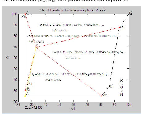
Restrictions (20) and points of an optimum in coordinates {x1, x2} are presented on figure 1.
Figure 1. Pareto's great number, SoS in two-dimensional system of coordinates
Step 2. We defined the worst unchangeable part of each criterion (anti-optimum):
X0
1={x1=25, x2=100, x3=25}, f 0 1=f1(X
0
1) = 11.0;
X0
2={x1=100, x2=100, x3=100}, f 0 2= f2(X
0
2)= -4270.9;
X0
3={x1=43.5, x2=20, x3=80}, f 0 3=f3(X
0
Vol. 3 Issue 4, April - 2017
www.jmess.org
X0
4={x1=100, x2=25, x3=100},f 0 4= f2(X
0
4)=-263.97. (Top index zero).
Step 3. The system analysis of a set of points, optimum according to Pareto is made, (i.e. the analysis by each criterion). In points of an optimum of X *={X
1*,
X2*, X3*, X4*} sizes of criterion functions of F(X*)=
K k
K q k q X
f 1,
, 1 *
)
( determined. Calculated a vector of D=(d1
d2 d3 d4)T - deviations by each criterion on an
admissible set of S: dk =fk*-fk0, k=1,4, and matrix of relative estimates of
(X*)= k K
K q k
q X
, 1 , 1 *
)
(
, where k(X)=(fk*-fk0)/dk.
F(X *)=
9.2 701.9 3704.1 11.0
95.1 724.7 3848.7 329.0
28.7 96.1 1200.0 374.0
209.6 127.1 2055.1 707.5
, D=
254.8
-639.7 3070.9
-696.5
,
(X *)=
1.0000 0.9644 0.1846 0
0.6628 1.0000 0.1375 0.4566
0.9232 0.0174 1.0000 0.5212
0.2132 0.0658 0.7216 1.0000
Discussion. The analysis of sizes of criteria in relative estimates showed that in points of an optimum of X *={X
1*, X2*, X3*, X4*} the relative assessment is equal to unit. Other criteria there is much less than unit. It is required to find such point (parameters) at which relative estimates are closest to unit. The step 4 is directed on the solution of this problem.
Step 4. Creation of -problem is carried out in two stages: originally the maximine problem of optimization with the normalized criteria is under construction:
o =
x max
k
min k(X), G(X)0, X 0,
which at the second stage was transformed to a standard problem of mathematical programming ( -problem):
o = max, (21) at restrictions
-o *
o
f f
- f
1 1
1 2 1 2
1
1...+0.014*x *x ...-0.07*x ...
x * 11.55 + 50.0
0, (22)
-o *
o
f f
- f
3 3
3 2 1 2
1
1...-0.002*x *x ...-0.0032*x ...
x * 0.118 -55.71
0, (23)
-o *
o
f f
- f
2 2
2 2 1 2
1
1+....-0.0519*x *x ...+0.0066*x ...
x * 0.7359 53.87
0, (24)
-o *
o
f f
- f
4 4
4 2 1 2
1
1...-0.0048*x *x ...+0.012*x ...
x * 0.2967 -25.6484
0, (25)
01, 25x1100, 25x2100, 25x3100, (26)
where the vector of unknown had dimension of N+1: X={x1, … , xN, }.
Step 5. Solution of a -problem. For the solution of a -problem we use the function fmincon(…), [10]:
[Xo,Lo]=fmincon('Z_TehnSist_4Krit_L',X0,Ao,bo,A eq,beq,lbo,ubo,'Z_TehnSist_LConst',options).
As a result of the solution of a vector problem of mathematical programming (16)-(20) at equivalent criteria and -problem corresponding to it (21)-(26) received: Xo={Xo, o}={Xo={ x
1=33.027, x2=69.54,
x3=25.0, o=0.4459}} - an optimum point – design
data of technical system, point Xo is presented in
figure 1; fk(Xo), k=1,K - sizes of criteria
(characteristics of technical system): {f1(Xo)=321.5,
f2(Xo)=2901.7, f3(Xo)= 370.2, f4(Xo)= 19.1}; (27)
k(Xo), k= 1,K - sizes of relative estimates: {1(Xo)=0.4459, 2(Xo)=0.4459, 3(Xo)=0.4459,
4(Xo)=0.9609}; (28)
o=0.4459 is the maximum lower level among all
relative estimates measured in relative units: : o=min
(1(Xo), 2(Xo), 3(Xo), 4(Xo))=0. 4459. A relative
assessment - o call the guaranteed result in relative
units, i.e. k(Xo) and according to the characteristic of technical fk(Xo) system it is impossible to improve, without worsening thus other characteristics.
Discussion. We will notice that according to the theorem 2 [5, 234 p.], in Xo point criteria 1, 2, 3 are
contradictory. This contradiction is defined by equality of 1(Xo)=2(Xo)=3(Xo)=o=0.4459, and other criteria an inequality of {4(Xo)=0.9609}>o.
Thus, the theorem 2 [5, 234 p.] forms a basis for determination of correctness of the solution of a vector task. In a vector problem of mathematical
programming, as a rule, for two criteria equality is carried out: o=
q(Xo) = p(Xo), q, p K, XS, (in our example of such criteria three) and for other criteria is defined as an inequality: o
k(Xo) k K,
qpk.
Step 6. Creation of geometrical interpretation of results of the decision in three to measured system of coordinates
In an admissible set of points of S formed by restrictions (26), optimum points X1*, X2*, X3*, X4* united in a contour, presented a set of points,
optimum across Pareto, to SoS . For specification of
border of a great number of Pareto calculated
additional points: X12o , X13o , Xo42, X34o which lie between the corresponding criteria. For definition of a point of X
o
12 the vector problem was solved with two criteria
(21), (22), (23), (26). Results of the decision:
X12o ={80.78 25.0 55.89}, o(Xo
12)=0.9264;
F12 ={656.2 1426.0 101.7 142.7};
L12 = {0.9264 0.9264 0.0261 0.4761}.
Vol. 3 Issue 4, April - 2017
www.jmess.org
X13o ={93.29 87.49 100.0}, o(Xo
13)=0. 7173;
F13 = {510.6 3924.4 543.8 206.2};
L13 = (0.7173 0.1128 0.7173 0.2267};
Xo42={25.0 29.92 25.0}, o(Xo
42)=0. 9301;
F42 = {374.3 1414.5 114.0 27.0};
L42 = {0.5217 0.9301 0.0454 0.9301}
Xo43={25.0 100.0 56.02}, o(Xo
43)=0. 8366;
F43 = {42.0 3757.6 695.4 25.0};
L43 = {0.0445 0.1672 0.9541 0.9541};
Points: X12o , Xo13, Xo42, Xo43 are presented in figure 1. Coordinates of these points, and also
characteristics of technical system in relative units of
1(X), 2(X), 3(X) , 4(X) are shown in figure 2 in three measured space {x1, x2, }, where the third axis of - a relative assessment.
Figure 2. The solution of -problem in three-dimensional system of coordinates of x1, x2 and
C. Decision-making on the basis of technical system model at the set priority of criteria
2 Algorithm. The decision in problems of vector optimization with a criterion priority
The solution of a vector problem (16)-(20) with a criterion priority was submitted as sequence of steps.
Step 1. We solve a vector problem with equivalent criteria. The algorithm of the decision is presented in section 3.2. Numerical results of the solution of a vector task are given above. Pareto's great number of SoS lies between optimum points X
1 *Xo
13X * 3X
o
43 X * 4X
o
42 X
* 2X
o
12X1 *.
We will carry out the analysis of a great number of Pareto SoS. For this purpose we will connect auxiliary points: Xo12, X13o , Xo43, Xo42, with a point Xo which
conditionally represents the center of a great number of Pareto. As a result have received four subsets of points
XS oq SoS, q= 4 ,
1 . The subset of S1o SoS is characterized by the fact that the relative assessment of
1 ≥2,3, 4, i.e. in the field of S first criterion has a
priority over the others. Similar to So2, S3o, So4,- subsets of points where the second - the fourth criterion has a priority over the others respectively. Set of points, optimum across Pareto we will designate So=So
1 S
o
2
So3 So4 . Coordinates of all received points and relative estimates are presented in two-dimensional space in fig. 1. These coordinates are shown in three measured space {x1, x2, } from a point of X*
4 in fig. 2 where the third axis of - a relative assessment. Restrictions of a set of points, optimum across Pareto, in fig. 2 it is lowered to -0.5 (that restrictions were visible). This information is also a basis for further research of structure of a great number of Pareto. The person making decisions, as a rule, is the designer of technical system. If results of the solution of a vector task with equivalent criteria don't satisfy the person making the decision, then the choice of the optimal solution is carried out from any subset of points of So1, So2, So3, So4..
Step 2. Choice of priority criterion ofqK. From the theory (see the theorem 2 [10]) it is known that in an optimum point of Xo always there are two most inconsistent criteria, qK and vK for which in relative units exact equality is carried out: o=
q(Xo) =p(Xo), q,
vK, XS, and for the others it is carried out inequalities: o
k(Xo) kK, qvk.
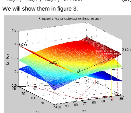
In model of technical system (16)-(20) and the corresponding -problem (21)-(26) such criteria are the first, second and third:
o=
1(Xo)= 2(Xo)=3(Xo)=0.4459. (29)
We will show them in figure 3.
Figure 3. The solution of -problem (1, 2, 3 criterion) in three-dimensional system of coordinates
Vol. 3 Issue 4, April - 2017
www.jmess.org As a rule, the criterion which the decision-maker
would like to improve gets out of couple of
contradictory criteria. Such criterion is called "priority criterion", we will designate it q=2K . This criterion is investigated in interaction with the first criterion of
k=1K.
On the display the message is given:
q=input ('Enter priority criterion (number) of q =') - Have entered: q=2.
Step 3. Numerical limits of change of size of a priority of criterion ofq=2K are defined.
For priority criterion of q=2 numerical limits in physical units upon transition from a point of an optimum of Xo to the point of X*
q received on the first
step are defined. Information about the criteria for q=2 are given on the screen:
f q(Xo) =2901.68 fq(X) 1200.0=fq(X*q
*
k
), qK. (30)
In relative units the criterion of q=2 changes in the following limits:
q(Xo) =0.4459q(X)1= q(X*q
*
k
), q=2K.
These data it is analyzed.
Step 4. Choice of size of priority criterion. qK. (Decision-making). The message is displayed: "Enter the size of priority criterion fq=" – we enter, for example, fq =1600.
Step 5. Calculation of a relative assessment.
For the chosen size of priority criterion of fq =1600 the relative assessment is calculated:
q=
o q * q
o q q
f f
- f f
=1200.0 4279.9 4279.9 -1600
=0.8697, (31)
which upon transition from Xo point to X*
q according to
(28) lies in limits:
0. 4459 =2(Xo) 2=0.86972(X*2)=1, qK..
Step 6. Calculation of coefficient of linear approximation.
Assuming linear nature of change of criterion of fq(X) in (30) and according to a relative assessment of
q(X), using standard methods of linear approximation, we will calculate proportionality coefficient between q(Xo), q, which we will call :
=
) (X λ ) (X λ
) (X -λ λ
o q * q q
o q q
=
4459 . 0 1
4459 . 0 8697 . 0
=0. 7649, q=2. (32)
Step 7. Calculation of coordinates of priority criterion with the size fq.
Assuming linear nature of change of a vector of
Xq={x
1 x2}, q=2 we will determine coordinates of a
point of priority criterion with the size fq =1600 with a relative assessment (31):
Xq={x
1 =Xo(1) + (X*q(1) - Xo(1))
x2 =Xo(2) + (X*q(2) - Xo(2))}.
where Xo={x
1=33.02, x2=69.54}, X*2={x1=25, x2=25}.
As a result of calculations we have received point coordinates:
Xq={x
1=26.88, x2=69.54}. (33)
Step 8. Calculation of the main indicators of a point of Xq.
For the received Xq point, we will calculate:
all criteria in physical units fk(Xq)={fk(Xq), k=1,K}:
f(Xq)={f
1(xq)=386.5, f2(xq)=1651.5, f3(xq)=137.9,
f4(xq)=26.1};
all relative estimates of criteria q ={q
k, k=1,K}, k(Xq)=
o k * k
o k q k
f f
- f X f
)
( , k=1,K
K
,1
:
k(xq)={1(xq)=0.5392, 2(xq)=0.853, 3(xq)= 0.0827,
4(xq)=0.9334};
vector of priorities Pq ={pq
k=
) (X λ
) (X λ
q k
q
q , k=1,K}:
Pq=[p2
1 =1.5820, p 2
2=1.0, p 2
3=10.3123, p 2
4=0.9139];
minimum relative assessment: minLXq=min(LXq): minLXq=min(k(Xq)) = 0.0827;
relative assessment taking into account a criterion priority:
oo=min (p2 1 1(X
q) =0.7564, p2 22(X
q) =0.7564, p2 3
3(Xq) =0.7564 , p244(Xq)) =0.7564).
Any point from Pareto's set Xto={ot , Xot }So can
be similarly calculated.
Analysis of results. The calculated size of criterion fq(Xot ), qK is usually not equal to the set fq.
The error of the choice of fq=|fq(Xot ) - fq| =|1651.5- 1600|=51.5 is defined by an error of linear
approximation, fq%= 3.2%.
In the course of modeling parametrical restrictions (20) can be changed, i.e. some set of optimum decisions is received. Choose a final version which in our example included from this set of optimum decisions:
parameters of technical system Xo={x
1=33.03,
x2=69.54, x3=25.0};
the parameters of the technical system at a given priority criterion q=2: Xq={x
1=26.88, x2 =35.47,
Vol. 3 Issue 4, April - 2017
www.jmess.org
IV. GEOMETRICAL INTERPRETATION OF RESULTS OF THE DECISION IN THREE TO MEASURED SYSTEM OF COORDINATES IN PHYSICAL UNITS
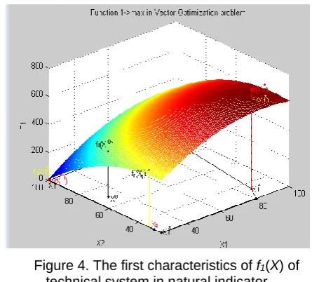
We represent these parameters in a
two-dimensional x1, x2 and three dimensional coordinate system x1, x2and in Fig.1, 2, 3, and also in physical units for each function f1(X), … , f4(X) on Fig. 4, ... , 7,
respectively.
The first characteristic f1(X) in physical units show
in Fig. 4.
Figure 4. The first characteristics of f1(X) of
technical system in natural indicator
In point Xo, Xq of the second characteristic of f 2(X) will assume to the look presented in figure 5.
Figure 5. The second characteristics of f2(X) of
technical system in natural indicator
In point Xo, Xq of the third characteristic of f
3(X) will assume to the look presented in figure 6;
Figure 6. The third characteristics of f3(X) of technical
system in natural indicator
In point Xo, Xq of the fourth characteristic of f 4(X) will assume to the look presented in figure 7;
Figure 7. The fourth characteristics of f4(X) of technical system in natural indicator
Collectively, the submitted version:
• point - Xo;
• characteristics of f1(Xo), f2(Xo), f3(Xo), f4(Xo); • relative estimates of 1(Xo), 2(Xo), 3(Xo) ,
4(Xo);
• maximum orelative level such that o k(Xo)
kK
- there is an optimal solution with equivalent criteria
(characteristics), and the procedure for obtaining an acceptance of the optimal solution with equivalent criteria (characteristics).
• point – Xq;
• characteristics of f1(Xq), f2(Xq), f3(Xq), f4(Xq); • relative estimates of 1(Xq), 2(Xq), 3(Xq) ,
4(Xq);
• maximum orelative level such that o k(Xq)
Vol. 3 Issue 4, April - 2017
www.jmess.org - there is an optimal solution at the set priority of the
second criterion (characteristic) in relation to other criteria. Procedure of receiving a point is Xqadoption
of the optimal solution at the set priority of the second criterion.
Theory of vector optimization, methods of solution of the vector problems with equivalent criteria and given priority of criterion can choose any point from the set of points, optimum across Pareto, and show the optimality of this point.
CONCLUSIONS
The problem of adoption of the optimum decision in difficult technical system on some set of functional characteristics is one of the most important tasks of the system analysis and design. In work the new technology (methodology) of creation of mathematical model of technical system in the conditions of
definiteness and uncertainty in the form of a vector problem of mathematical programming is presented. For the first time in domestic and foreign literature, we have submitted the theory of vector optimization and methods for the choice of any point, from Pareto's great number. The principles of an optimality of a point are shown in the theory, first, at equivalent criteria, secondly, at the set criterion priority. These methods can be used at design of technical systems of various branches: electro technical 2, aerospace,
metallurgical, etc. At creation of characteristics in the conditions of uncertainty regression methods of transformation of information are used. The methodology of modeling and adoption of the
optimum decision is based on normalization of criteria and the principle of the guaranteed result (maxmin). Methods allow solving vector problems at equivalent criteria and with the set criterion priority. Results of the decision are a basis for decision-making on the studied technical system on all set of point’s optimum across Pareto. This methodology has system
character and can be used when modeling both technical and economic systems. Authors are ready to participate in the solution of vector problems of linear and nonlinear programming.
REFERENCES
[1] Mashunin, Yu. K, Methods and Models of Vector Optimization, Nauka, Moscow, 1986, 146 p. (in Russian).
[2] Mashunin, Yu. K., and Levitskii, V. L., Methods of Vector Optimization in Analysis and Synthesis of
2 We mention the work of V.L. Levitskii “Simulation and Optimization of Parameters of Magnetoelectric Linear Inductor Electric Direct Current Motor” [7, p. 50–120]. It deals with designing an augmented electric motor (AEM) with its model reduced
to vector mathematical programming problem (1)–(5). The vector of design parameters X = (X1, …, X5) consisted of X1 for
the air clearance δ, X2 for the tooth pitch, X3 for the number of teeth, X4 for the height of the concentrator, and X5 for the pole
overlap coefficient. The vector of design criteria F(X) = (f(X), p(X), η(X), …) included f(X) for the nominal towing force,
Engineering Systems. Monograph. DVGAEU, Vladivostok, 1996. 131 p. (in Russian).
[3] Mashunin, Yu. K. Solving composition and decomposition problems of synthesis of complex engineering systems by vector optimization methods. Comput. Syst. Sci. Int. 38, 421–426, 1999.
[4] Mashunin K. Yu. , and Mashunin Yu. K. Simulation Engineering Systems under Uncertainty and Optimal Descision Making. Journal of Comput. Syst. Sci. Int. Vol. 52. No. 4. 2013. 519-534.
[5] Mashunin Yu. K. Control Theory. The mathematical apparatus of management of the economy. Logos. Moscow. 2013, 448 p. (in Russian).
[6] Mashunin Yu. K., and Mashunin K. Yu. Modeling of technical systems on the basis of vector optimization (1. At equivalent criteria). International Journal of Engineering Sciences & Research Technology. 3(9): September, 2014. P. 84-96.
[7] Mashunin Yu. K., and Mashunin K. Yu. Modeling of technical systems on the basis of vector optimization (2. with a Criterion Priority). International Journal of Engineering Sciences & Research Technology. 3(10): October, 2014. P. 224-240.
[8] Yu. K. Mashunin, K. Yu. Mashunin. Simulation and Optimal Decision Making the Design of Technical Systems // American Journal of Modeling and Optimization. 2015. Vol. 3. No 3, 56-67.
[9] Yu. K. Mashunin, K. Yu. Mashunin. Simulation and Optimal Decision Making the Design of Technical Systems (2. The Decision with a Criterion Priority) // American Journal of Modeling and Optimization. 2016. Vol. 4. No 2, 51-66.
[10] Ketkov Yu. L., Ketkov A. Yu., and Shul’ts M. M., MATLAB 6.x.: Numerical Programming. BKhV_Peterburg, St. Petersburg, 2004. 672 p. (in Russian).
p(X) for the nominal power, η(X) for the nominal efficiency and so on, ten indices in total. The central orthogonal plan of the
second order was used to construct the dependencies of f on the listed design parameters X [7, p. 96]. The work “…Multiobjec_
tive Optimization of Static Modes of Mass_Exchange Processes by the Example of Absorption in Gas Separation” [15] is an
example from another industry. Thus, experimental data both from the AEM problem and from similar ES of other industries