Paper 06-2009-1

UDC: 556.536:519.876.5(282.243.743)

Modeling of Flow in River and Storage with Hydropower Plant, Including

The Example of Practical Application in River Drina Basin

M. Arsić1_{*, V. Milivojević}2_{, D. Vučković}3_{, Z. Stojanović}4_{, D. Vukosavić}5

Institute for Development of Water Resources “Jaroslav Černi”, 80 Jaroslava Černog St., 11226

Beli Potok, Serbia. e-mail: 1_{[email protected],} 2_{[email protected],}

3_{[email protected],} 4_{[email protected],} 5_{[email protected]}

*Corresponding author

Abstract

Goal of the mathematical modeling and simulation of a physical system is to provide the user with the relevant information used in design and/or management decision-making. Spatial decomposition formulates the mathematical models of water flow with the parameters and rules describing the water route. Calculation of the inlet hydrograph transformation along the river section and storage was exercised by virtue of the hydrological methods that are actually a simplified solution of the fundamental differential equations of flow. Calculation of discharge through hydro-technical structures, such as spillways, foundation outlets etc., are shown in hydraulic equations or water level-discharge relations. Storage management includes direct or indirect planning of the hydropower plant operation, as well as meeting other water management requirements. Hydropower plant work plan can be created on the basis of water level management in the storage or desired electricity generation. Efficient numerical algorithms provide for processing of input event series and initial values that describe the state in the river and storage, resulting in the series of events on all important locations of the physical system. An example illustrates the application of the mathematical models of flow in the river, wave transformation in the storage and electricity generation calculation. The example covers the part of the River Drina basin between the profiles of “Zvornik” HPP and “Bajina Bašta” HPP.

Keywords: Flow modeling, river, storage, hydropower plant, calculation algorithms

1. Introduction

The goal of the mathematical modeling and simulation of a physical system is to provide the user with the relevant information used in design and/or management decision making. Results can be used for perception of the effects of decisions on a real system under regular or extraordinary hydrological conditions.

Modeling of the hydropower system is the part of broader and more complex water flow modeling that starts with the rainfall-runoff process, continues with the flow in the rivers and storages and ends with the flow through hydro-technical structures and hydropower plants. Present paper deals with hydropower system with the river section, storage and the hydropower

plant. Formation of the inflow from the catchment area is the topic of Prodanović et al. (2009).

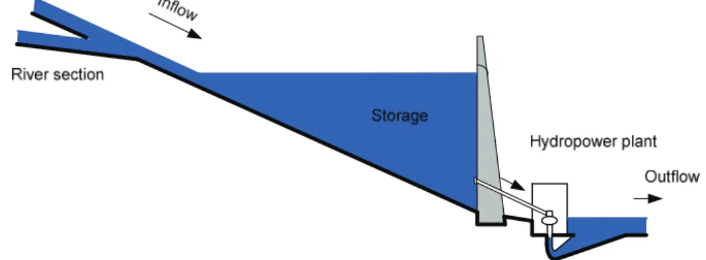
Therefore, the subject physical system includes the river section and profiles with known water levels and discharges, storage with known water level-volume relation and hydropower plant operation which has an influence on the level in the storage. System modeling is the mathematical interpretation of water flow through the natural watercourses and storages and water flow through outlet structures and the hydropower plant.

The following figure presents an outline of the subject hydropower system.

Fig. 1. Outline of the hydropower system (river section, inflow, storage, hydropower plant and outflow)

The following text will present the spatial decomposition, theoretical background of applied mathematical models and the example of application of the model of the hydropower system on the River Drina basin.

2. Spatial decomposition and general rules

Modeling of the nature requires proper knowledge of the complexity of natural phenomena, as well as the adequate sense of the method and the degree of approximation used to model physical processes. Mathematical models are the models of water flow on large and complex areas, including: water entry into the system, flow in open courses, flow through outlet structures on dams and flow and electricity generation in hydropower plants.

Spatial decomposition should be performed in line with realistic geo-morphological and hydro-meteorological spatial features. Decomposition is performed by defining the river sections and control structures in the flow, such as dams or measurement profiles. Spatial decomposition introduces several mathematical models to simulate naturally and artificially formed water flows as follows:

 Flow in open courses,

 Transformations in the storage,

 Flow through foundation outlets on dams,

 Leakage on dam sites and

 Flow and electricity generation in hydropower plants.

Mathematical models components used for spatial decomposition contain parameters describing their behavior, procedures of inlet hydrograph transformation into outlet hydrograph and the rules of water delivery and demand-forwarding to water users described in Hydro-Information System “Drina”.

For the subject hydropower system, composed of river flow, storage and hydropower plant, components of the mathematical model are as follows:

 Storage hydro-profile,

 Hydro-node,

 Open course flow and

 Plant.

In terms of modeling, the storagehydro-profile is a collection of structure’s mathematical

models linked by mutual links, relations and rules into a model unit. Broadly speaking, the structural elements of the storage hydro-profile are as follows:

 Storage,

 Spillway,

 Foundation outlet,

 Tailrace and

 Water losses in the storage (due to seepage and evaporation).

The following figure shows a decomposition of the storage profile.

The storage is a confined area where the water level and volume are changing within the defined range. Water inflow can come from the watercourse, underground flows and hydro-technical structures (for example, tunnels). Water discharge from the storage can be: through the hydropower plant, over the spillway, through the foundation outlet, due to seepage, due to evaporation off the water area and due to water release for water users (such as water supply, irrigation, navigation locks etc.).

Fig. 2. Decomposition of the storage hydro-profile (storage evaporation, discharge over the spillway, discharge through the foundation outlet, discharge through the tailrace, leakage)

The following figure shows a decomposition of a spillway into the spillway fields.

Fig. 3. Decomposition of the spillway structure into spillway fields

Foundation outlet is used for storage emptying, water level maintenance in the storage and water release to downstream users. Foundation outlet, as an entity, is used for modeling water release from the storage for use by downstream users (guaranteed discharge, water used for water supply, irrigation etc.).

The following figure shows a decomposition of the foundation outlet structure into individual outlets.

Fig. 4. Decomposition of the foundation outlet structure into individual outlets

Tailrace, in terms of modeling, is the part of the river bed used as a collection point for all storage outlets (flows over the spillway, flows through the foundation outlet, leakage, discharge through the hydropower plant with the powerhouse at the base of the dam etc). In the tailrace the dependency between water level and water flow is created, and it is the point where the ecologically guaranteed discharge is to be let out.

Hydro-node is the spot along the river course where several river courses meet (a confluence), where the river course bifurcation starts (flow through river branches, flow around river islands etc.), or the location of control point (water-measurement station). Hydro-nodes are the structures with known level-grams, hydrographs or discharge curves. Boundary conditions can also be set on hydro-nodes.

Following figure shows a decomposition of tributary to main course.

Fig. 5. Decomposition of the confluence of rivers

River sections can be linked by a hydro-node or dam structure. Linking several river

sections together will form an open flow network. Open flow model is used for water flow

separately or just the entire plant. Following figure shows a decomposition of the hydropower plant into individual units.

Fig. 6. Decomposition of the open flow between the hydro-node and the storage

Fig. 7. Decomposition of the hydropower plant into individual units

Management of the complex hydropower and water-management system includes the ability to meet the requirements of the electricity generation and transmission system, meet a series of limitations on control profiles, provide a good navigation environment and riverbanks stability etc. Additionally, the operation of individual objects in the cascaded hydropower system must be coupled.

Electricity generation and transmission system requirements are set by the daily production plan, i.e. the total daily electricity generation in the hydropower plant or on each individual unit. Hydropower plant rulebook can define production ranges along the timeline.

Simulation model is a collection of mathematical models of spatial decompositions that unify mathematical functions and input data. Water transfer between individual mathematical models in the simulation model is performed in line with the rules integrated in the software modules.

Water transfer rules are set in line with the water flow laws of nature and according to the water user request.

Input data for calculation in the simulation model are the parameters and time series. Parameters describe general behavior of the model, while the time series describe the model behavior at any given time.

3. Mathematical models

3.1. Modeling of the flow in the river and storage

Inlet hydrograph routing is a process of the hydrograph “advancing” and change along the water course. Hydrological analyses should, therefore, apply relevant computing methods for occurrence time and form of the inlet hydrograph.

In natural watercourses and canals, water is temporarily captured during the inlet hydrograph propagation. The result of that is the transformation of the hydrograph form. Effect of the capturing in a specific river sector is the function of the volume of the space where the water is captured.

Obviously, the larger the volume of space between the inlet and outlet profile of the river sector, the bigger are differences in the form of inlet and outlet hydrographs.

Flood routing calculation procedures are the mathematical methods of setting the intensity and velocity of flow routing changes in water propagation through the river or storage.

Procedures are divided into:

 Hydrological and

 Hydraulic ones.

Hydrological procedures use the principle of continuity and the link between the outlet spot and temporary storage for excess water during the discharge growth.

Hydraulic procedures use numeric solving of differential equation of instationary flow (Saint-Venant equation), as follows:

 Continuity equation:

0

Q A

q

A t

 _ _{ }

  (1)

 Dynamic equation:

1 1

te

A V V V

I I

B x



 

  

  _  _   

wherein:

 Q – discharge,

 q – lateral inflow,

 A – area of the discharge section,

 V – flow velocity,

 x – distance,

 g – gravity acceleration,

 B – flow width,

 t – time,

 ξ – loss coefficient,

 I0 – river bed bottom slope and

 Ite – free water surface slope.

Solving of the equations requires defined calculation elements that can be subjected to algebraic approximations. Calculation of the unsteady flow requires data both on upstream and downstream boundaries, as well as defined internal boundary conditions (confluence, dams, side spillways etc.). Modeling of unsteady flow involves problems in calculation, such as sensitivity to approximation errors and time dimension of the problem. Calculation complex as

this one is justified in case of big river hydropower systems such as system of “Đerdap HPP”

(described in Grujović et al. 2009).

Hydraulic procedures, generally speaking, may be considered as more accurate than the hydrological ones. Specialized literature, for example, indicates that the hydrological methods result in higher peak discharges than the ones resulting from the application of hydraulic methods. Application of hydraulic procedures, on the other hand, is far more complex that the application of hydrological, even when simplifications and approximations are introduced. It is also considered that the accuracy of hydrological methods is sufficiently high for application in many practical examples.

In case of hydropower systems with poor hydrological and morphological data, simplified methods are often used. Hydrological methods of computation of inlet hydrograph transformation are focused on water redistribution computing in the storage, and friction forces that can impact water pools circulation, are not taken into consideration. Problem solving by these methods is based only on solving the continuity equation. Hydrological methods of routing are further divided into:

 Methods of calculation of inlet hydrograph transformation through the storage and

 Method of calculation of inlet hydrograph routing along the natural water courses or

channels.

3.1.1. Balancing models of hydrograph transformation through the storage

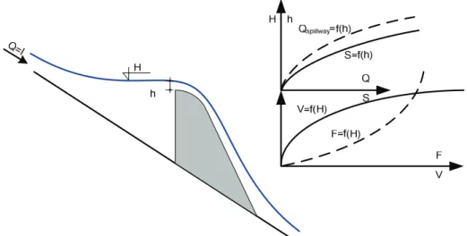
Inlet hydrograph transformation through the storage is the simplest form of inlet hydrograph routing. Due to small velocity of water flow, one can assume that the water level in the storage is horizontal. Conclusion is that the water volume in the storage and the discharge can be directly expressed by water level in the storage (Prohaska (2001), Jovanovic (2002) and US

Simultaneous solving of the continuity equation and the volume–discharge functional dependency results in numeric solution of the inlet hydrograph transformation.

The following dependencies are required for the calculation:

 Volume–level of water in the storage, S = f(H) and

 Discharge–level of water in the storage, Q = f(h)

Figure 8 is a schematic description of the storage with the basic parameters.

Fig. 8. Schematic description of the storage with the basic parameters

Variable V in the previous figure designates the water volume in the storage and the variable S designates part of the storage volume used for inlet hydrograph transformation.

Continuity equation reads:









1 1

2 Ii Ii   t 2 Oi Oi  t SiSi (3) wherein:

 I – inflow into the storage,

 O – outflow from the storage,

 S – water volume in the storage and

 Δt – time step.

Indices (i – 1) and i designate the start and end of the discretization period Δt.

Equation (3) has two unknowns, Oi and Si, and cannot be solved without the introduction of

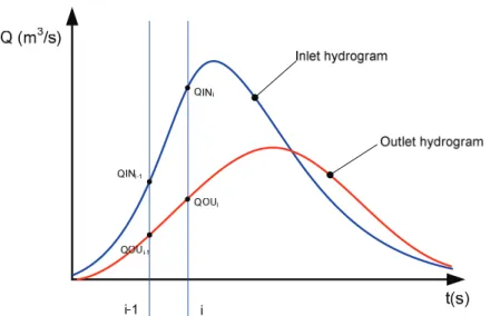
Fig. 9. Schematic presentation of inlet hydrograph transformation through the storage (sum of storage inlets, sum of storage outlets)

This specific case uses an independent equation that is characterized by dynamic dependency between water volume in the storage and the storage outflow. Equation includes the variables such as the height of spilling jet, hydropower plant water demand in time, water release to downstream users etc:

0

( ) j

i j i

O 



Water volume in the storage is also dependent on the water level in the storage:

 

S S H (5)

At the calculation time “i”, known values are the inflows Ii and Ii-1, water volume in the

storage Si-1 and outflow from the storage Oi-1. Outflow Oi is obtained by solution of equations

(1) and (2).

3.1.2. Balance models of hydrograph transformation along the river section

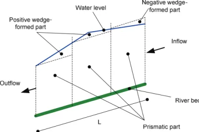
Fig. 10. Elements of water volume on the river sector during the inlet hydrograph propagation time (inlet discharge, positive wedge-formed part, flow line, negative wedge-formed part, outlet

discharge, river bottom, prismatic volume part)

During the water level increase, in the river sector positive wedge-formed parts of the volume appear. However, when the inlet hydrograph decrease starts to be more intensive than the outlet hydrograph drop, negative wedge-formed parts of the volume appears. Procedure of calculation of inlet hydrograph routing requires adequate realization of volume impact, particularly regarding its wedge-formed part. This is the reason to integrate into the routing the calculation of discharges on both inlet and outlet profiles of the sector.

“Muskingum” Method

“Muskingum” method is broadly applied in hydrological practice. The method was designed by McCarthy in 1936, within the study of floods in the River Muskingum basin. The method uses a linear dependency between the water volume and discharges on the entry “I” and exit “O” profiles of the river sector with two parameters K and X (Prohaska (2001), Jovanovic (2002) and US Army Corps of Engineers).

In the “Muskingum” method, water volume can be expressed as a weighted function of mean discharges on the boundary profiles of the sector:

[ ( - ) ]

S  K X I   l X O (6)

wherein:

 S – volume,

 K – parameter with a time dimension,

 X – non-dimensional constant,

 I – discharge on the inlet sector and

 O – discharge on the outlet sector.

parameter K and constant X can be determined by the graph that demonstrates the dependency between volume S and the “weighted” discharge on the outlet sector, computed by the equation;

( - )

O  I X  l X O (7)

Graph S = f(O) is formed for various constant X values. The “Muskingum” method assumes that the dependency between the volume and the “weighted” discharge is linear. For the accepted value of constant X, which yields the lowest spread of the experimental spots and the equation of line running through their center, parameter K is computed using the curve slope, i.e.: S K O  

 (8)

Dimension of parameter K depends upon the dimension of volume and discharge. If the

volume is in m3_{/day, and the discharge is in m}3_{/s, K will have the dimension of the day.}

Continuity equation:









1 1

2 I I   t 2 O O  t S S (9)

in combination with equations (7) and (8) creates the following equation for inlet hydrograph routing calculation under the “Muskingum” method:

2 2 0 1 1 1 2

O I C I C O C (10)

where in C0. C1 and C2 are the coefficients calculated by the following equations:

0 0.5_{( - ) 0.5}t K X

-C

K l X t

  



    (11)

1 0.5_{( - ) 0.5}t K X

C

K l X t

    

   (12)

2 K l X_{( - ) 0.5}( - ) - 0.5 t

C

K l X t

  



    (13)

In previous equations, Δt is the time discretization period.

Sum of coefficients C0. C1, and C2 must be 1. Water volume on the sector can be calculated

by means of known values of inlet and outlet hydrographs using the equation:





Calculation starts at the time when the inlet and outlet discharges are equal, i.e. when the inflow from the inter-catchment is minor.

Value of discretization period is set by the conditions: 2

t K X

    (15)

For the registered values of inlet and outlet hydrographs, parameters X and K are determined, whereby the value of parameter X should be between 0 and 0.5. Values of accepted parameters can be used only for waves similar to those used to calibrate the model.

For the calculation of the flow along the river section under the “Muskingum” method, input data are the hydrograph at the start of the section and parameters K and X. Calculation result is the hydrograph at the outlet of the river section.

“Muskingum-Cunge” method

French hydraulics expert Cunge showed in 1969 that the “Muskingum” method is a special case of the discretized equation of the kinematic wave. He formulated the expressions for parameters X and K as dependent upon the river course features in a way that the values are changed along the course and calculated at any time per transversal profiles. Introduced variable are:

 θ that represent the weighted factor and

 c = (g · A / B)0.5 _{that represents wave velocity.}

For values X = θ and K = (Δx / c), wherein Δx is the distance between two transversal

profiles on the river section, coefficients C0. C1, and C2 are equal for both methods.

Equation development for inlet hydrograph routing calculation in the “Muskingum-Cunge”

method and expression for parameter X (in fact θ) can be derived:

0 1

1

2 2 _d

Q X

I B c x

 

  _{ }

   

  (16)

wherein:

 Q0 – arbitrary discharge,

 Id – local slope and

 B – width of the flow.

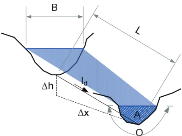
The following figure shows geometric variables of the river section.

Parameter K is the time of wave propagation, while parameter X is the factor of wave attenuation, because it is physically linked to watercourse features by means of the geometry and friction.

Values of both parameters of the “Muskingum-Cunge” method are adapted during the calculation to flow conditions and section characteristics. The method is of more general character than the original “Muskingum” method with fixed parameters values, related to the river section.

Calculation of the steady non-uniform flow level line results in initial dependencies c =

c(Q0), for a series of arbitrary discharges. These values are the base of flow calculation.

Calculation is stable for values 0 < θ < 0.5, whereby the wave attenuation increases with

the decrease in value of θ. Upper limit of the profiles distance is set by the condition that θ

must not be negative or on the basis of empirical criterion:

2 p t x c



 (17)

Fig. 11. Geometric variables of the river section

For the calculation of the flow along the river section by application of the “Muskingum– Cunge” method, input data are the hydrographs at the start of the section and c is wave velocity. Calculation result is a hydrograph at the outlet of the river section.

“Muskingum” and “Muskingum-Cunge” methods cannot describe the impact of dead zones on flow, because they are based on the assumption of the uniform flow. These methods are also not applicable if the flow through the channel exceeds its flow capacity and if the water spill has occurred, because the model parameters values are considered constant (in case that a major change of velocity occurs and that also reflects on the value of parameter K).

“Muskingum-Cunge” method is suitable for calculation of the unsteady flow in torrent flows without the back-water impact coming from tributaries, dams etc. According to the experience, this method can be successfully used for torrent flows with bottom slope higher than 0.1% and inlet hydrographs with steep short branch of the hydrograph (30-60 minutes).

3.2. Modeling of the structures on the dam

Water evacuation over the spillway and through the foundation outlets is applied if the inflow in the storage is higher than the installed discharge of the hydropower plant, or if high waters are expected under the inflow forecast: hence, in order to prevent damages caused by high water, water is to be timely evacuated from the storage. Water evacuation from the storage is also applied when water is needed for downstream water management users. Capacity of evacuation/outlet structures is defined according to the level of headwater and the opening of the spillway gate, or the opening of the foundation outlet gate.

Calculation of the electricity generation in the hydropower plant is performed on the basis of discharge through the power plant, head and input data that describe the operational features of the hydropower plant as a whole or each unit individually. According to the method of assignment of input data in the power plant mathematical model, power calculation models of different level of detail are applicable.

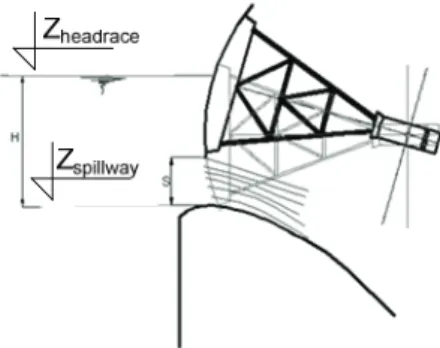
3.2.1. Spillway

Fig. 12. Spillway with the lifted gate

Spillway performance is defined by the following variables:

 ESC – elevation of the spillway cut-off,

 N – number of spillway fields and

 S (m) – level of gate lifting/lowering.

Characteristics of a spillway field are presented by the discharge curves given in the form of parameters for different values of the gate positions.

Discharge through the gate is determined for a known value of the headwater level and a known position of the gate. Total spillway flow is the sum of spillway flows through the individual spillway fields.

Operational methods of the spillway with gates can be modeled as:

 Defined outflow through the individual gates during the time of calculation and

 Defined degree of gate opening during the time of calculation.

In the first case, water outflow through spillway fields is defined for each time step during the calculation, while in the second the water flow through each spillway field is defined by the degree of gate opening for each time step during the time of calculation.

Spillways without gates have no physical means of regulation. The following figure is a schematic presentation of the spillway without gates.

Generally speaking, capacity of a spillway without gates is dependent upon its geometric and hydraulic characteristics and the height of spillway jet. Overflow is unavoidable when the storage water level exceeds ESC. Amount of the spilled water is determined by the spilling curve, as the function of water level in the storage equals:

( _hr )

k k

Q_spill  f Z (18)

wherein:

 k

spill

Q – splillway flow through kth _{spillway field,}

 k – spillway field index,

 k

hr

Spillway curve is a sum of overflows for all spillway fields. If spillway fields have different ESCs, than the applied variable is the one on the spillway field where its value is at the minimum.

Fig. 13. Spillway without gates – spilling over the dam body

Input data for the overflow calculation are: spilling curve, elevation of the spillway cut-off and spillway operational method. Calculation results are the height of the spillway jet and the discharge through the spillway during the time of calculation.

3.2.2. Foundation Outlet

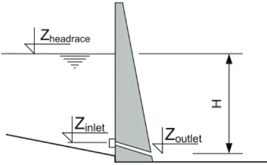
Foundation outlet can be used to model storage emptying, maintaining desired water level in the storage and water release for use by downstream users. The following figure is a schematic presentation of the foundation outlet.

Z

Z

Zheadrace

Fig. 14. Foundation outlet

Operation of the foundation outlet is described by the following variables: upstream and downstream elevation of the foundation outlet (axis elevation) and discharge curve.

Foundation outlets can be with and without regulation. Discharge through the foundation outlet is determined according to the water level in the storage and the discharge curve is read. If the foundation outlet has no regulation gate, the characteristic is presented only for the case of a fully lifted gate on the foundation outlet. If the foundation outlet is fitted with the regulation gate, its characteristic is presented in the form of parameters for various openings of the regulation gate.

Operational method of the foundation outlet can be modeled as:

 Defined outflow through each individual foundation outlet during the time of calculation

and

 Defined degree of gate opening for each individual foundation outlet during the time of

In the first case, water flow through the foundation outlets is defined for each time step during the time of calculation, while in the other case water outflow through each foundation outlet is defined by the degree of gate opening for each time step.

Input parameters for the discharge calculation are: discharge curve, elevations of the foundation outlet and operational method of the foundation outlet. Result of the calculation is the outflow through the foundation outlet.

3.2.3. Leakage

Process of leakage through the body and sides of the dam is unavoidable and is dependent upon the water level in the storage. Leakage curve can be determined by measurement, but in practice it is often determined by the balance equation of the storage. Result of leakage calculation is the hydrograph of leakage.

3.3. Modeling of the storage-type hydropower plant

Modeling of the hydropower plant operation is based on data describing operational characteristics of the units and the desired mode of operation. Specific modes of hydropower

plant operation with the calculation algorithms are presented in Vukosavić et al. (2009). The

present paper deals with power plant modeling in general.

The following figure is a schematic presentation of hydropower plant disposition.

Data used to describe power plant are: number of units, transformer efficiency and efficiency accounting for plant’s own consumption. The unit is divided into the intake system, turbine and generator. Intake system is described by the typical discharge and head losses for that discharge. Turbine characteristics are in the form of operational diagrams. Generator characteristics are presented in the form of nominal power of the generator and generator efficiency as a function of its load.

Depending on the level of calculation detail, i.e. method of presentation of performance of units, turbines, generators and intake structures, as well as on the time discretization, the following operational modes of the hydropower plant were formed:

 Modes with assignment of the daily electricity generation for the hydropower plant as a

whole,

 Modes with assignment of the hydropower plant power during any hour of the simulation,

 Modes with run-off-river operation of the hydropower plant and

 Modes with explicit assigning of the power, i.e. discharge, for each unit in the plant during

any hour of the simulation.

These modes enable short-term or long-term management of different hydropower plants types. Short-term management is a calculation for a period of several days, with the hourly discretization, and the long-term management is a calculation for a period of more then one year, with daily discretization.

In terms of modeling, plant can have two operational modes:

 With the planned water level in the storage, when the electricity generation is calculated

according to the available discharge from the storage, and

 With assignment of the targeted electricity generation.

Fig. 15. Schematic presentation of the hydropower plant (headwater level, operating water level, tailwater level and gross head)

Hydropower plant operation in the first mode is dictated by water level management in the storage. Input data are the inflow into the storage and the planned (targeted) water level in the storage, and the result is electricity generation. If the assignment of targeted storage water level is such that it cannot be fully achieved by the hydropower plant operation, a deviation from the targeted water level occurs and evacuation/outlet structures – foundation outlets and spillway are engaged.

In the second operational mode, the plan dictates the water volume in the storage. Input data are the inflow into the storage and planned (targeted) electricity generation, and the calculation result is the water level in the storage. If the assignment of electricity generation is such that it cannot be fully achieved by the hydropower plant operation, a deviation from the plan occurs and evacuation/outlet structures – foundation outlets and spillway are engaged.

Calculation results are dependent of the applied mode presented by the following values in general terms:

 Electricity generation of the hydropower plant, i.e. each unit,

 Power realized by the hydropower plant, i.e. each unit,

 Water discharge through the hydropower plant, i.e. each unit,

 Fulfillment of demands,

 Specific water consumption etc.

4. Application of the models in the HIS application library

circulation in the hydro-systems and one can draw a conclusion that the main challenge in formulation of complex catchment models is the creation of the interaction between the models treating only individual events in the catchment area. A realistic approach to modeling, aimed at integrated catchment area management, is actually the linking of different models and their joint

execution with full interaction during the simulation. Paper Milivojević et al. (2009a) presents

some of the standards that enable the creation of complex catchment area models. Although they do not restrict models to water resources domain, the standards are somewhat specialized and they can not be treated at the level of general systems and model and simulation specifications, such as time discrete models, continuity models or event based simulations. Therefore, many models based on these general principles must be subsequently “introduced” to the system, what requires experts and time; this is something often not justified if the models of individual parts of the catchment area are not overly complex. In view of the clear heterogeneity of the addressed models in terms of time and spatial discretization, limitations of the model’s continuity and time specification are to be overcome, which directly points the way to the model specification with discrete events.

Simulation of the presented models is performed by application of efficient numeric algorithms that enable the processing of input event series and initial situation values in the river and storage, resulting in event series on all major spots of the physical system. Numeric

algorithm is presented in Paper Milivojević et al. (2009a), i.e. library of classes in Paper

Milivojević et al. (2009b) that described mathematical models and respective simulation

models. Class for each structure is derived from the atomic model class including adaptation of standard functions. In the case of the storage hydro-profile, input ports (natural and artificial) are defined to determine the inflow and information on requirements imposed on the storage, as well as output ports delivering water to the structures (conditionally and unconditionally).

A similar procedure is also performed for all flow structures. This leads to formulation of the classification library of hydro-system structures used for model coupling. Further hierarchical model coupling of the mentioned entities enables formation of the simulation model of one part of the basin, or of the entire basin, for different build-up levels and different assumptions on structure performance (both for existing and future structures).

This method was used to develop a certain number of simulation models, paper Divac et al. (2009), applied within broader IT solutions for hydro-information systems of major basins. A hydro-information system is a distributed information system supporting basin water management, cf. Divac et al. (2009). A simulation model is the fundamental part of the complex software and is a core of a distributed information system that supports basin water management. As one of the system inputs is presented in the form of basin outflow and user requirements, the model incorporates all relevant line forms of the flow: flow through natural watercourses according to their morphological features, flow through the structures (dam spillways and outlets, hydropower plants, tunnels, canals, pipelines etc.). Change in flow conditions is modeled as time function as a result of management decisions (delivery, priorities and limitations, harmonized with defined electricity generation and water demand as a function of the system situation parameters). As a support to decision making, the model was developed for calculations in daily and hourly time discretization.

Full control over the model formation by simulation and result analysis is in the user interaction with the software package. Even though a major portion of the process of structure creation, automatic formation of coupled models and parameters and inputs setting is automatic, the user can exert an impact on various parameters and, thus, analyze the problem in interactive

manner (Milivojević et al. 2009b). Common user interface was developed to serve as an

software, guiding the user through the simulation process with a series of views and dialogues in an interactive and intuitive manner.

Besides the structure of the complex model, it is also possible to change all parameters of the real models and, thus, deviate from the pre-defined values. Pre-defined parameters values simplify the creation of initial models since the structures are assigned with parameters corresponding to existing hydro-structures, or planned in case of future situation description.

5. Example of practical application of the hydropower system mathematical model

The following example will illustrate the use of the mathematical models: flow in the river - “Muskingum-Cunge”, wave transformation in the storage, hydropower plant model. The example is related to the River Drina basin between “Zvornik” HPP and “Bajina Bašta” HPP profiles.

Fig. 16. Analyzed area – spatial decomposition

Illustration of the mentioned models of flow in the river, storage and hydropower plants is executed by the simulation model “Drina” HIS, developed by the Institute for Development of

Water Resources “Jaroslav Černi”. Simulation model includes the models of surface and

underground outflows, flow through the river section, transformations in the storage, flow through the dam evacuation/outlet structures and flow through the hydropower plant.

The following figure shows the mathematical model of the analyzed area of the example hydropower system.

Model spatial decomposition was exercised on the following parts /structures:

 “Zvornik” HPP,

 Storage “Zvornik” with a tailrace,

 Section of the river course from the end of “Zvornik” storage to “Mala Dubravica” profile,

 Section of the river course from “Mala Dubravica” profile to “Mihaljevići” profile,

 Section of the river course from “Mihaljevići” profile to “Ljuboviđa” profile on the

Ljuboviđa River and

 Profile replacing the “extracted” part of the basin, i.e. exit of the “Bajina Bašta” HPP.

The following figure is schematic presentation of spatial decomposition.

Fig. 17. Schematic presentation of model spatial decomposition (river section, storage and tailrace profile)

Major part of the river discharge downstream from “Bajina Bašta” HPP is directly related to the operational regime of the “Bajina Bašta” HPP. Lateral inflow to the River Drina on the

subject inter-catchment, in terms of modeling, is “captured” on “Mihaljevići”, “Mala

Dubravica” profiles and “Zvornik” HPP profile. In addition to the model parameters, these discharges are taken as the calculation data.

5.1. Calibration of the flow in the river and storage model

Calibration of the parameters of the mathematical model for the analyzed space was performed: rainfall-runoff, flow in the open course and wave transformation in the storage. Calibration of

the parameters was performed the period from July 1st_{, 2000 to March 1}st_{, 2002. Calibration was}

based on the following data:

 Recorded total discharge on “Bajina Bašta” HPP profile (Qpowerplant, Qspillway, Qoutlet),

 Computed inflow from the inter-catchment by the rainfall-runoff model,

 Recorded water level in the “Zvornik” storage and

 Recorded total discharge on the “Zvornik” profile.

The following morphological data were available for calibration procedure: volume curve of the “Zvornik” storage and cross-section profiles on the river sections from the “Bajina Bašta” storage to the “Zvornik” storage.

Discharge curves on a hydro-node were computed on the basis of measured and computed values of the water level and discharge, or they were computed by application of the Shezy equation. Initial value of wave-propagation velocity (a parameter of the “Muskingum-Cunge” method) was determined using the specialized literature sources.

0 200 400 600 800 1000 1200 01 .01. 2000 01 .03. 2000 01 .05. 2000 01 .07. 2000 01 .09. 2000 01 .11. 2000 01 .01. 2001 01 .03. 2001 01 .05. 2001 01 .07. 2001 01 .09. 2001 01 .11. 2001 Q[ m3 /s ] МЕРЕНО СИМУЛИРАНО

Fig. 18. Comparative presentation of measured and simulated values on “Zvornik” profile (measured and simulated discharges)

Comparative presentation of measured and simulated values indicates satisfactory correspondence between the measured and simulated hydrographs. The difference in water amounts is obviously a consequence of rough balancing measurement of the inflow on the dams.

For the adopted parameter values of the model that were confirmed by the calibration results, the operation analysis of the calculation model of the storage (with the hydropower plant) can be applied under predefined hydrological conditions.

5.2. Presentation of input data

The following example illustrates the adoption of HPP work plan for an assumed hydrological situation. Calculation model formation begins with the assignment of inflow hydrograph on

inlet profiles “Bajina Bašta”, “Ljuboviđa”, as well as of inter-inflows on profiles “Mihaljevići”,

“Mala Dubravica” and “Zvornik” storage profile.

The following figure is an illustration of the inlet hydrograph on the “Bajina Bašta” storage profile.

Fig. 19. Assignment of inlet hydrograph on “Bajina Bašta” storage profile

Q(m

3 /s)

Time (day)

Parameters of the “Muskingum-Cunge” model are assigned, i.e. calculated, for each river sector determined by an upstream and a downstream hydro-node.

The following figure illustrates the model parameters: wave propagation velocity hydrograph and morphological features of the river section.

All predefined profiles or confluence of river sections have a discharge curve as an input parameter. Shezy equation was used to compute discharge curves of certain profiles, wherein the Manning’s friction coefficient was taken from the profile for which the Republic Hydro-Meteorological Service had determined the discharge curve.

Fig. 20. River course parameters

The following figure illustrates the discharge curve on the control profile “Mihaljevići”.

Fig. 21. Discharge curve on profile “Mihaljevići”

Fig. 22. Dialog boxes: storage hydro-profile (left) and storage (right)

Parameters of the hydropower plant for selected operational model were illustrated in the following figure. Present example illustrates the hydropower plant operational Mode 1 “Assignment of Daily Electricity Generation, HPP Optimum Operation”.

Fig. 23. Parameters of the hydropower plant and HPP operational model

Requirement value is formed on the basis of expected inflow to the storage, targeted water level in the storage and targeted electricity generation. The following figure presents the demand.

5.3. Calculation results

The following results are calculated for the predefined input data of the mathematical model. River section flow result is presented in the form of inlet and outlet hydrograph.

Fig. 25. Calculation results on the river section downstream from the “Bajina Bašta” HPP profile

Previous diagrams indicate transformation of the inlet hydrograph, i.e. the attenuation of the peak value and the lag time of the inlet hydrograph.

Hydrograph transformation in the storage and the impact of “Zvornik” HPP operations on storage water level can be presented by level-gram as well as by inlet and outlet hydrographs.

Fig. 26. Storage calculation results

Fig. 27. Spillway calculation results

Discharge though the power plant and electricity generation under presented HPP operational regime are presented in the following diagram.

Calculation results are also the generated power, operation time etc.

In the illustrated computation example, “Zvornik” storage has a relatively small volume. Result of this and analyzed inflow to the storage is previously presented (realized) HPP operational plan.

Fig. 28. Calculation of HPP operational results

6. Conclusions

Present paper explains the principles of the hydropower system modeling by spatial decomposition, components of the mathematical model and calculation algorithm.

Dam structure modeling (spillways and foundation outlets) is performed in order to compute water evacuation from the storage, aimed at protection against high waters or for the needs of downstream water users.

Storage management in hydropower systems is closely related to HPP operation. The main reason for this is the retentive capacity of the storage that also impacts the choice of the HPP modeling method.

There are several mathematical models of storage-type hydropower plant that enable short-term or long-short-term management. Model selection is also directly related to the level of detail in the calculation, i.e. the method used to present performance of the units, turbines, generators and intake conduits, as well as to time discretization.

A computation example was used to illustrate the application of mentioned computation models in the software used on the River Drina basin. Experts in water management, storage management and electricity generation planning, as well as designers, can use the applied models and this software to make and test their design decisions.

References

Divac D, Grujović N, Milivojević N, Stojanović Z, Simić Z (2009), Hydro-Information Systems

and Management of Hydropower Resources in Serbia, Journal of the Serbian Society for

Computational Mechanics, Vol. 3, No. 1

Grujović N, Divac D, Stojanović B, Stojanović Z, Milivojević N (2009), Modeling of

One-Dimensional Unsteady Open Channel Flows in Interaction with Reservoirs, Dams and

Hydropower Plant Objects. Journal of the Serbian Society for Computational Mechanics,

Vol. 3, No. 1

Institute for Development of Water Resources “Jaroslav Černi” (2001), Studija varijantnih

scenarija razvoja “Hidrosistema Drina”, I faza, Belgrade

Institute for Development of Water Resources “Jaroslav Černi” (2002), Hidro-Informacioni

Sistem “Trebišnjica”, Simulacioni Model Verzija 2.1, Belgrade

Institute for Development of Water Resources “Jaroslav Černi” (2005), Hydro-Information

System “Drina”,Simulacioni Model Verzija 2.0. Belgrade

Institute for Development of Water Resources “Jaroslav Černi” (2006), Hydro-Information

System “Drina”,Simulacioni Model Verzija 2.1, Belgrade

Jovanović M (2002), Regulacija reka, Belgrade

Milivojević N, Grujović N, Stojanović B, Divac D, Milivojević V (2009), Discrete Events

Simulation Model Applied to Large-Scale Hydro Systems. Journal of the Serbian Society

for Computational Mechanics, Vol. 3, No. 1

Milivojević V, Divac D, Grujović N, Dubajić Z, Simić Z (2009), Open Software Architecture for

Distributed Hydro-Meteorological and Hydropower Data Acquisition, Simulation and Design

Support. Journal of the Serbian Society for Computational Mechanics, Vol. 3, No. 1

Prodanović D, Stanić D, Milivojević N, Simić Z, Stojanović B (2009), Modified Rainfall–

Runoff Model for Bifurcations Caused by Channels Embedded in Catchments. Journal of

the Serbian Society for Computational Mechanics, Vol. 3, No. 1

Prohaska S (2001), Hidrologija, Belgrade

Vukosavić D, Divac D, Stojanović Z, Stojanović B, Vučković D (2009), Several Hydropower

Production Management Algorithms. Journal of the Serbian Society for Computational

Mechanics, Vol. 3, No. 1