Evolving Water Resources Systems: Understanding, Predicting and Managing Water–Society Interactions Proceedings of ICWRS2014, Bologna, Italy, June 2014 (IAHS Publ. 364, 2014).
3
Variational data assimilation with the YAO platform for
hydrological forecasting
AMARA ABBARIS
1, HAMMOUDA DAKHLAOUI
2,3, SYLVIE THIRIA
1&
ZOUBEIDA BARGAOUI
21 LOCEAN, Université Pierre et Marie Curie, Institut Pierre Simon Laplace, 4, place Jussieu 75252 Paris Cedex 05, France
2 LMHE, Université Tunis El-Manar, Ecole Nationale d’Ingénieurs de Tunis, BP 37, 1003 Tunis le Belvédère Tunisie. 3 ENAU, Université de Carthage, 20 Rue El Qods, 2026 Sidi Bou Saïd, Tunis, Tunisie
Abstract In this study data assimilation based on variational assimilation was implemented with the HBV hydrological model using the YAO platform of University Pierre and Marie Curie (France). The principle of the variational assimilation is to consider the model state variables as control variables and optimise them by minimizing a cost function measuring the disagreement between observations and model simulations. The variational assimilation is used for the hydrological forecasting. In this case four state variables of the rainfall– runoff model HBV (those related to soil water content in the water balance tank and to water contents in rooting tanks) are considered as control variables. They were updated through the 4D-VAR procedure using daily discharge incoming information. The Serein basin in France was studied and a high level of forecasting accuracy was obtained with variational assimilation allowing flood anticipation.
Key words variational assimilation; YAO; HBV model; hydrological forecasting; optimisation; SCE-UA
INTRODUCTION
Floods represent one of the most destructive hazards to human lives and properties. To mitigate such a hazard, lots of research has focused on improving real-time monitoring and flood forecasting (Droegemeier et al. 2000). Numerous techniques were developed to improve hydrological forecasting, especially high flood prediction. Data assimilation was found to be one of the main tools to achieve this task (Seo et al. 2003, 2009, Ouachani et al. 2007, Lee et al. 2012). The 4D-Var method (variational data assimilation) is used in geophysics, applied to physically-based numerical models, in particular in meteorology (Schlatter 2000) and oceanography (Nodet 2007). It consists of estimating the control parameters of a direct numerical model (the hydrological model in our case), by minimizing a cost function quantifying the mismatching between the forecast values and actual observations. Gradient methods are adopted for the minimisation process. At University Paris VI, the research team of LOCEAN has developed a computation platform named YAO implementing the 4D-Var technique (Nardi et al. 2009). In this study, it is proposed to apply variational assimilation using the YAO framework to perform hydrological forecasting. Thus, the rainfall–runoff model HBV is adopted as a forecasting tool whose state variables are updated by 4D-Var to reduce the forecasting uncertainty.
METHODS AND TOOLS The HBV Rainfall–Runoff Model
The HBV model is one of the most successful conceptual rainfall–runoff models that has been applied in more than 30 countries. In the current study, a lumped modelling is adopted. The main model outputs are daily mean flows (m3/s) as well as daily actual evapotranspiration (mm/day). The
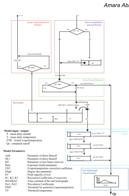
principal water balance components of the HBV model are snow accumulation and melt, actual evapotranspiration and infiltration evaluation, soil humidity evolution, and water transfer through soil (Fig. 1). A further description of the HBV model version used in this study can be found in Dakhlaoui and Bargaoui (2013). The model includes several state variables evolving continuously, which decide the flows values. They are mainly the soil moisture level (SW), the water level in the rooting tanks (STW1, STW2, and STW3) and the depth of the snow accumulated (SD).
Fig. 1 HBV model structure.
Variational assimilation
Variational assimilation (4D-VAR) (Le Dimet et al. 1986) considers a physical phenomenon described in space by one, two or three dimensions and its time evolution. It thus requires the knowledge of a direct dynamical model M, which describes the time evolution of the physical phenomenon. M allows connecting the geophysical variables studied with observations. By varying some geophysical variables (control variables), assimilation seeks to infer the physical variables that led to the observation values. The basic idea is to determine the minimum of a cost function J that measures the misfits between the observations and the model estimations. Due to the complexity related to the nonlinearity of this function, the desired minimum is classically obtained by using gradient methods, which implies the use of the tangent linear and the adjoint models of M. The latter and the former are derived from the equations of the direct model M. The adjoint model estimates changes in the control variables in response to a disturbance of the output values calculated by M
(here HBV equations). It is therefore necessary to proceed backwards to tangent linear calculations, which means using the transpose of the Jacobian matrix. When observations are available, the adjoint allows minimizing of function J, and finding the values of the control variables (in our case:
SW, STW1, STW2 and STW3). YAO
YAO provides a framework helping the implementation of the adjoint model using programming based on a general formalism decomposition of complex systems into a modular graph (Nardi et al.
2009, http://www.locean-ipsl.upmc.fr/~yao/). The graph is composed of modules connected by nodes and representing the numerical model. Each module is composed of an elementary function specific to the dynamic model, which is differentiable. YAO compiles and generates an executable that can compute the direct model M, the tangent linear model M and the adjoint model Mt. An
interface with a quasi Newton optimizer called M1QN3 (Gilbert and Le Marechal 1989) is used to minimize the cost function. YAO, using forward and backward integrations of M and its adjoint, yields the derivatives.
Qper1=PER1*STW1
PD PD
STW1
STW2
STW3 Smelt=DD(T-TT)
SW PWP FC
No Yes
SD
No Yes
Pe=Smelt+PDI
Qs=Auft*(Pe-HL1)
PE=Pe-Qs PE=Pe
Qs Maxbas Pe <HL1
if T <TT
SW<PWP Yes
No ETR=ETP
ETR=ETP*SW/PWP
Q1=K1*STW1(1+K0)
Q2=K2*STW1
Q3=K3*STW3 Qper2=PER2*STW2
HSW=PE* (1-(SW/FC)**Beta) 1-HSW
QD
: Parameter of direct Runoff : Parameter of direct Runoff : Parameter of non linear reservoir : Exponent model parameter : Evapotranspiration correction coefficient : Degree day parameter
: Field capacity of soil : Recession Coefficients of reservoirs : Time constant of the unit hydrograph : Percolation Coefficients : Threshold for potential evapotranspiration : Threshold temperature
Auft HL1 K0 Beta CEF Degd FC K1, K2, K3 MAXBAS Per1, Per2 PWP TT
Model Parameters Model input / output:
P : mean daily rainfall T : mean daily temperature ETR : Actual evapotranspiration Qs : simulated runoff
Routine and melt Routne
Direct Runoff Routine
Soil routine
Runoff generation routine
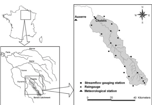
Fig. 2 Location of the Serein catchment in the Seine basin.
DATA
The variational assimilation was applied to predict the floods of the Serein (France). It is a tributary of the Seine (Fig. 2). It is mainly situated in a rural zone. It presents an elongated form with an area of 1120 km2. The streamflow gauge is situated at Chabelis and began to work in 1955. The daily
mean flow is about 7.9 m3/s which is the equivalent of 255 mm/year. The annual mean rainfall is
about 850 mm.
METHODOLOGY OF HYDROLOGICAL FORECASTING 4D-VAR
The 4D-Var was considered to assimilate outflows and to predict floods. Four model state variables are considered a priori as control variables: the soil moisture (SW) and the levels of water in the rooting tanks (STW1, STW2 and STW3) (Fig. 1). In fact, several studies proved the importance of such variables (Zehe et al. 2005, Lee et al. 2012).
Forecasting tests were performed under perfectly known rainfall. The control variables are updated every time step by the assimilation of the hydrological data of the n previous time steps (days). The forecasting is applied for the pthtime step (day). Several combinations of assimilation windows width (n) and forecast lead time (p) were tested.
The effect of these decision variables on the quality of forecasting was studied. The Nash criterion (Nash and Sutcliffe 1970) was considered to evaluate the forecasting performance. In addition, we have evaluated the precision of the forecasting procedure to predict the peak flows. To that purpose, three objectives were targeted: reconstitute the occurrence, the amplitude and the timing of peaks. The first objective is quantified using a binary criterion. In effect, when the forecasting procedure generates a peak that matches to an observed one (regardless of the magnitude), this criterion takes the value “yes”, and if no peak is generated this criterion takes the value “no”. We note that this criterion is estimated with an objective manner by the observer (expert hydrologist). For the amplitude, we compare the amplitude of the matched observed and simulated peaks. We quantify the relative error between the observed and simulated peak flows. For the timing, we evaluate the delay (in days) between the observed and the simulated peak. The evaluation is assumed negative in the case of premature forecast and positive for delayed predicted peaks.
RESULTS AND DISCUSSION Calibration of HBV model
there is some difficulty for the model to reconstitute peak flows, which justify the potentiality for data assimilation to improve this situation.
Hydrological forecasting
The model parameters applied to run forecasting were those obtained by calibration in the previous section. Two periods were selected for the forecasting experiences, the first from 17 January 2009 to 27 February 2009 and the second from 9 March 2008 to 14 May 2008. The former contains five peaks, while the latter contains nine peaks, the highest values occurred on 26 January 2009 and on 24 March 2008, respectively. Figures 3, 4 and 5 show examples of hydrographs of the variational assimilation forecasts against the observed flows and the simulated runoff using the HBV model (called raw model simulation).
In Fig. 3, the assimilation period was considered equal to n = 3 days and the forecast lead time to p = 1 day. It results in an important improvement in the forecasting accuracy compared to the raw model. In effect, the Nash of the forecasted flow is increased to 0.93 (0.70 for the raw model). In addition, four of the five peak flows were detected by the forecasting procedure. Particularly the peak of 5 February 2009, which was not detected by the raw model, is predicted in the present experience (Table 1). We also note that the forecasted recession flows are underestimated compared to the observed ones. In effect, the recession is more rapid in forecasting than in realty.
For the second observation period, with a forecast lead time of n = 1 day and an assimilation period of p = 3 days (Fig. 4), the Nash of predicted flow is about 0.95. All peak flows are detected, but with a relative error of up to 12%. We also find a very important improvement of the
Fig. 3 Evolution of streamflow predicted (fine dished line) compared to those obtained with HBV simulation (bold dished line) and observed streamflow (continuous line) at the outlet of the Serein for the observed period 17 January 2009 to 27 February 2009 with 3 days assimilation and 1 day forecast lead time. SW, STW1, STW2 and STW3 are updated with assimilation (HBV without assimilation Nash = 0.70, Assimilated flow Nash = 0.93.
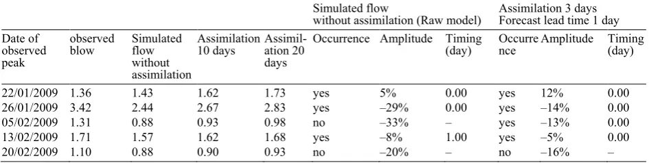
Table 1 Comparison of peak flows (occurrence, amplitude and timing) of stream flow forecasted with 3 assimilation and 1 day forecast lead time, to those obtained with HBV simulation with the observed stream flow at the outlet of the Serein, for the observed period of 17 January 2009 to 4 March 2009.
Simulated flow
without assimilation (Raw model) Assimilation 3 days Forecast lead time 1 day
Date of observed peak
observed
blow Simulated flow
without assimilation
Assimilation
10 days Assimil-ation 20
days
Occurrence Amplitude Timing
(day) Occurrence Amplitude Timing (day)
22/01/2009 1.36 1.43 1.62 1.73 yes 5% 0.00 yes 12% 0.00
26/01/2009 3.42 2.44 2.67 2.83 yes –29% 0.00 yes –14% 0.00
05/02/2009 1.31 0.88 0.93 0.98 no –33% – yes –13% 0.00
13/02/2009 1.71 1.57 1.62 1.68 yes –8% 1.00 yes –5% 0.00
20/02/2009 1.10 0.88 0.90 0.93 no –20% – no –16% –
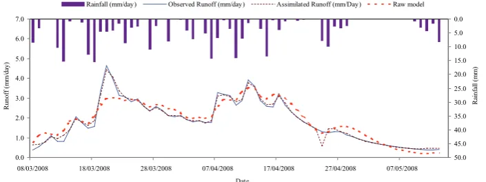
Fig. 4 Evolution of streamflow predicted (fine dished line) compared to those obtained with HBV simulation (bold dished line) and observed stream flow (continuous line) at the outlet of the Serein for the observed period 9 March 2008–14 May 2008, with 3 days assimilation and 1 day forecast lead time. SW, STW1, STW2 and STW3 are updated with assimilation. HBV without assimilation Nash = 0.87, Assimilated flow Nash = 0.95.
Fig. 5 Evolution of streamflow predicted (fine dished line) compared to those obtained with HBV simulation (bold dished line) and observed streamflow (continuous line) at the outlet of the Serein for the observed period 9 March 2008–14 May 2008, with 2 days assimilation and 1 day forecast lead time. SW, STW1, STW2 and STW3 are updated with assimilation. HBV without assimilation Nash = 0.87, Assimilated flow Nash = 0.98.
reconstitution of the most important peak flow, as well as the one ranked at second position; they were not detected without the updating process. However, a tendency to underestimate the recession time was monitored. In effect, the predicted recession segments are lower than the observed ones, especially for the second half of the observed period.
When the assimilation period is decreased to p = 2 days (n = 1 day), a spectacular improvement in prediction performance is noted (Fig. 5). The Nash of predicted flow reaches 0.98. We observed a quasi-perfect prediction of peak flow amplitude, timing and occurrence. The rising and recession segments of predicted flows match better to observations.
For the forecast lead time (p = 2 days), augmenting the assimilation window to n = 3 days, we note an important decline of the prediction accuracy (Table 2). In effect, the variational assimilation results in a lower Nash (= 0.81) than in the case without state variables updating (Nash = 0.87). There is an important discordance between the predicted peak flows and the observed ones, as well as in amplitude, timing and occurrence. Although the variational assimilation could estimate the peaks amplitude of the most important floods, it presents a lag of 1 day in the timing of peaks. For the other secondary events, the variational assimilation has difficulty in catching up with the observations, and sometimes completely misses the observed.
In this series of tests with Serein, we note that the accuracy of prediction decreases along the observed period. Generally the assimilation improves forecasting compared to HBV model simulation (raw model). The forecast lead time of p = 1 day and the assimilation period n of two days give the best results. In fact, the time differences and similarities among the forecasts may be seen best in this case. For other combinations of assimilation windows and forecast lead times, we
0.0 1.0 2.0 3.0 4.0 5.0 6.0 7.0
09/03/2008 19/03/2008 29/03/2008 08/04/2008 18/04/2008 28/04/2008 08/05/2008
Date
Runoff (m
m/
da
y)
0
5
10
15
20
25
30
35
40
Ra
inf
all (
mm/d
ay
)
Rainfall (mm/day) Simulated Runoff (raw model! mm/day)
Assimilated runoff (mm/day) Observed Runoff (mm/day)
0.0 1.0 2.0 3.0 4.0 5.0 6.0 7.0
08/03/2008 18/03/2008 28/03/2008 07/04/2008 17/04/2008 27/04/2008 07/05/2008
Date
Runoff (m
m
/da
y)
0.0 5.0 10.0 15.0 20.0 25.0 30.0 35.0 40.0 45.0 50.0
R
ain
fa
ll (
mm)
times, for the Serein.
Studied period Assimilation
period (days) Forecasting lead time (days) Nash of predicted flow Nash without assimilation (Raw model) 17 January 2009–
27 February 2009 3 1 0.93 0.70
9 March 2008–
14 May 2008 3 2 1 1 0.95 0.98 0.87
3 2 0.81
can deduce an over forecast and an under forecast some time severe. The worst results were obtained with n = 3 days assimilation and p = 2 days (Table 2).
CONCLUSION
According to this experience, the 4D-Var method and YAO as a tool are powerful for developing assimilation procedures. The methodology was to select the most sensitive state variables for updating with data assimilation. Several assimilation periods and forecast lead times were evaluated.
In the case of the Serein (1120 km2) using the daily time step, soil moisture content (SW) and
rooting tanks levels (STW1, STW2 and STW3) were adopted as control variables (four variables). A high level of forecasting accuracy was obtained with either 1 or 2 days anticipation of floods. The assimilation periods were 2 or 3 days. The forecasting accuracy was also evaluated with respect to both occurrence and timing of flow peaks. Of course, more and more experiments on other basins have to be achieved to confirm the success of the present experiments.
Acknowledgements Authors would like to thank IRSTEA for data. This work is part of the Tunisia– France scientific cooperation 2011−2014 program CMCU number 10G1102.
REFERENCES
Dakhlaoui, H., Bargaoui, Z and Bárdossy, A. (2012) Toward a more efficient Calibration Schema for HBV Rainfall-Runoff Model.
Journal of Hydrology 444–445, 161–179.
Dakhlaoui, H. and Bargaoui, Z. (2013) A hybrid SCE-UA-KNN Optimisation Algorithm applied to the calibration of Rainfall-Runoff Model. In: Calibration Theory and Application (ed. by Ikumatsu Fujimoto and Kunitoshi Nishimura). Nova Publication. ISBN: 978-1-62618-808-2
Droegemeier, K. K., et al. (2000) Hydrological aspects of weather prediction and flood warnings: Report of the 9th Prospectus Development Team of the US. Weather Research Program, B. Am. Meteorol. Soc. 81, 2665–2680.
Ide, K., et al. (1997) Unified Notation for Data Assimilation: Operational, Sequential and Variational. Special Issue. J. Meteorological
Society Japan 75, 181–189.
Lee, H., et al. (2012) Variational assimilation of streamflow into operational distributed hydrologic models: effect of spatiotemporal scale of adjustment. Hydrol. Earth Syst. Sci. 16, 2233–2251, www.hydrol-earth-syst-sci.net/16/2233/2012/ doi:10.5194/hess-16-2233-2012
Le Dimet, F.-X. and Talagrand, O. (1986) Variational Algorithms for Analysis and Assimilation of Meteorological Observations: Theoretical Aspects. Dynamic Meteorology and Oceanography 38.
Nardi, L., et al. (2009) YAO: a Software for Variational Data Assimilation using Numerical Models, Int. Conf. on Computational Science and its Applications, ICCSA 2009, Seoul, South Korea, June 2009, pp.Part II, 621–636, Series LNCS 5593. Nash, J. E. and Sutcliffe, J. V. (1970) River flow forecasting through conceptual models. 1. A discussion of principles. J. Hydrol.
10(3), 282–290.
Nodet, M. (2007) Variational assimilation of Lagrangian Data in Oceanography. SIAM Conference on Applications of Dynamical Systems.
Ouachani, R., Bargaoui, Z. and Ouarda, Taha (2007) Intégration d'un filtre de Kalman dans le modèle hydrologique HBV pour la prévision des débits. Hydrological Sciences Journal 52(2), 318–337. DOI: 10.1623/hysj.52.2.318.
Saltelli, A. (2008) Sensitivity Analysis. John Wiley & Sons Edition. USA.
Schlatter, A. W. (2000) Variational assimilation of meteorological observations in the lower atmosphere: A tutorial on how it works
Journal of Atmospheric and Solar-Terrestrial Physics 62(12), 1057–1070.
Seo, D.-J., Koren, V. and Cajina, N. (2003) Real-time variational assimilation of hydrologic and hydrometeorological data into operational hydrologic forecasting, J. Hydrometeorol. 4, 627–641.
Seo, D. J., et al. (2009) Automatic state updating for operational streamflow forecasting via variational data assimilation. Journal of
Hydrology 367, 255–275.
YAO Home Page http://www.locean-ipsl.upmc.fr/~yao/