ANALYSIS OF CITIES DATA USING PRINCIPAL COMPONENT
INPUTS IN AN ARTIFICIAL NEURAL NETWORK
Villuri Mahalakshmi Naidu1, Chekuri Siva Rama Krishna Prasad2, Manchikanti Srinivas3, Praveen Sagar4
1,2 National Institute of Technology, Warangal, India
3,4 GVP College of Engineering (Autonomous),Visakhapatnam, India
Received 21 September 2017; accepted 27 May 2018
Abstract: Trip rate is one of the transportation planning parameter. It is difficult to relate the amount of trips that originate in a study area and the amount of trips attracted towards that study area by conducting surveys regularly. The cost and time for each survey is not affordable. So considering Travel parameters and Land-use Parameters of an area relationship is established using Artificial Neural Network (ANN) against Trip Rates of that area. Involving more number of parameters has made computations to increase the complexity in analysis. So the data has been reduced in dimension using Principal Component Analysis and then Processed in an Artificial Neural Network. The original input data along with principal components (6PC, 5PC, 4PC and 3PC) data as input to the Artificial Neural Network (ANN) has been processed separately. The analysis has shown that 6PC as input to Artificial Neural Network(ANN) is yielding better explanation between independent and dependent variables (Trip Rate(all modes) and Trip Rate(motorised)).
Keywords:artificial neural network (ANN), principal component analysis (PCA), trip rate, trainlm,feed forward back propagation network.
1. Introduction
Every survey conducted in transportation planning has a large amount of data as outcome. Artificial Neural Network when employed for the purpose of data analysis involves higher number of inputs. The more the number of Inputs provided to an Artificial Neural Network the more number of calculations are carried out. It also takes more time for calculations. Principal Component Analysis is a data reducing technique which reduces the data into fewer number of inputs, without loss of information. It is also helpful in classifying data based on the variations in
23 Principal Components where the first 6 Principal Component explain 85- 90 percent of the Original data. So these 6 Principal Components are processed against Trip Rate (all-modes) and Trip rate (motorised) and compared with original data Inputs Vs Trip Rate (all-modes) and Trip rate (motorised) processed in Artificial Neural Network.
The methodology of principal components has been taken as established in (Paul et al.,
2013) and (Manage and Scariano, 2013). Artificial neural networks and training algorithm are well described in (Pham and Sagiroglu, 2001), (Sharma and Venugopalan, 2014) and (Aggarwal and Kumar, 2015). (Burns and Whitesides, 1993) explained the concept of patterns and application of feed-forward neural network. (Gevrey et al., 2003) demonstrated comparison of methods in neural network. (Lyons et al., 2001) explained the application of neural network to enhance the operation of pedestrians at mid-block signalized crossing. (Kadali et al., 2014) also described the evaluation of pedestrians at mid-block with the application of neural network. Based on these literature, for Artificial Neural Network modeling with Back propagation Algorithm and Trainlm training functions were used.
2. Methodology
Cities which are densely populated and have a major share of trips per day have been selected in this study. Data related to these 26 cities regarding various travel parameters and Land –use parameters have been obtained using various sources and surveys. Population (in lakhs according to Census 2001), Population Density, Trip length (km), Congestion index, Per capita income, Male%, and Female% are the travel parameters considered. Area (sq. km), Agricultural (sq.km), Water bodies and Coastal (sq.km), Residential (sq.km), Industrial (sq.km), Public and Semi-public (sq.km), Recreational (sq.km), Transport (sq.km), Commercial (sq.km) are the Land-use parameters considered. These Travel parameters and Land-use parameters are now reduced using Principal Component Analysis. These reduced inputs are made to establish a relationship between Trip Rate (all-modes) and Trip Rate (motorised).
The selected Travel parameters and Land-use parameters are considered as inputs to the artificial neural network.
Cities data is given in Tables 1 and 2.
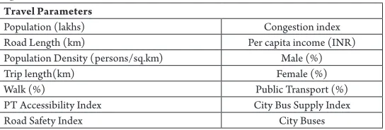
Table 1
Trip Rate Parameters
Travel Parameters
Population (lakhs) Congestion index
Road Length (km) Per capita income (INR)
Population Density (persons/sq.km) Male (%)
Trip length(km) Female (%)
Walk (%) Public Transport (%)
PT Accessibility Index City Bus Supply Index
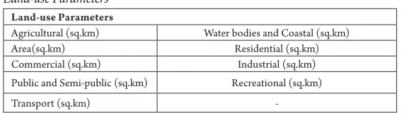
Table 2
Land-use Parameters
Land-use Parameters
Agricultural (sq.km) Water bodies and Coastal (sq.km)
Area(sq.km) Residential (sq.km)
Commercial (sq.km) Industrial (sq.km)
Public and Semi-public (sq.km) Recreational (sq.km)
Transport (sq.km)
-The step by step procedure adopted in the methodology is as shown below.
1. A feed-forward Back propagation Network is selected with Trainlm Training function.
2. Cities data is processed using Principal Component Analysis.
3. Principal Components are captured. The Components with more amount of information from the original data are selected.
4. The selected Principal Components and the corresponding target data (i.e., trip rate) are given as inputs to the selected Network.
5. The target data here are trip rates of the selected cities. Trip rates include motorised trips and person trips.
6. Data division is random and weights initialization is also random, controlled by a random number generator.
7. Neural network provides the results in the form of Mean Square Error (MSE) and Regression Value (R).
8. The complete data set is processed directly using the network and the results are observed.
9. Another set of reduced data obtained using the PCA is also processed using the same network and the results are compared.
3. Network Modelling
Fig. 1 is the proposed Network Architecture with PCA inputs. It has one Input layer, one Hidden Layer, One output layer. Input layer has 6 Neurons for the 6 principal Components. These 6 Inputs are connected to 6 Hidden layer neurons which are being
processed against the target data Trip Rate (all-modes) and Trip rate (motorised) separately. Here the network is trained for two conditions first against Trip-Rate (all-modes) and next against Trip rate (motorised).
Fig. 1.
Network Architecture with PCA Inputs
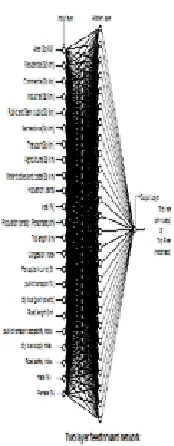
Fig. 2.
Fig. 2 is the proposed Network Architecture with original Inputs. It has one Input layer, one Hidden Layer, One output layer. Input layer has 23 Neurons for the 23 selected parameters. These 23 Inputs are connected to 24 Hidden layer Neurons. Which are
being processed against the target data Trip Rate (all-modes) and Trip rate (motorised) separately. Here the network is trained for two conditions first against Trip-Rate (all-modes) and next against Trip rate (motorised). Data size is as given in Table 3.
Table 3
Training and Testing Data Size
Input case Input Size Training Validation Testing
PCA 26 x 6 16 x 6 5 x 6 5 x 6
Original 26 x 23 16 x 23 5 x 23 5 x 23
4. Data Analysis Results
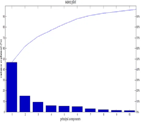
Fig. 3 is a combination plot between variance of each principal component and cumulative variance against each principal component. This shows how much information each
principal component carries out. Maximum information is explained by the first three principal components. So for the further analysis first six principal components are considered as they explain almost 90% of the data.
Fig. 3.
Fig. 4.
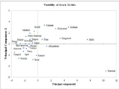
Scatter Plot of Parameters on PC-1 and PC-2
Bi-plot shown in Fig. 4 and 5 consist of the correlation between observations and variables i.e. correlation between a city and it parameters.
The dots represent the relative positions of cities with principal component one and two. Lines represent position of the Parameter with respect to principal component one and two. For clear understanding the position of cities are labeled and plotted.
Selecting a correlation value greater than 0.7 component one is closely related to area (sq. km), Trip length (kms), Public transport (%), city buses, Residential (sq.km), Industrial (sq. km), recreational (sq.km), Transport (sq.km) are positive towards component 1 indicating that each parameter grows with growth in one or two parameters. It also says that these parameters are interlinked. Variables that are positively correlated with component 2 is Male (%) and negatively correlated is female (%).
Fig. 5.
So in cities correlated well towards component 2 if male population increases more chances of female population to decrease as given in Table 4. Cities highly
correlated to component 1 are Mumbai, Delhi, Kolkata, Bangalore and Hyderabad. Cities highly correlated to component 2 are Chennai, Hyderabad, Kochi, and Madurai.
Table 4
Various Parameters related to Principal Components
PC-1 PC-2 PC-3
Population (In Lakhs-2001) Male % Population Density
Area (sq km) (-) Female %
-Trip Length (km) -
-Public Transport (%) -
-City Buses -
-residential(sq km) -
-Industrial(sq km) -
-Recreational(sq km) -
-Transport(sq km) -
-4.1. Training Results for Network with Original and Principal Components as Inputs
and Trip Rate (All-Modes) as Target
Fig. 6.
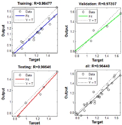
The resulting graph in Fig. 6 shows how the
training, testing, validation for data of original inputs against target data Trip Rate (all-modes). Mean square error is 0.075 in 2 epochs.
Fig. 7.
Performance of Network with R Value (R) (6-PCA Vs Trip Rate (All-Modes)
Fig. 7 shows training, testing, validation for data of original inputs against target data Trip Rate (all-modes) Mean square error is 0.007 in 2 epochs.
Comparative results of original and Principal Component Inputs Vs Trip Rate (all-modes) are tabulated in Table 5.
Table 5
Comparative Results for Trip Rate (All-Modes) as Target Data
Inputs Vs
all-modes R MSE epochs
PCA-6 0.96448 0.007 2
PCA-5 0.95046 0.013 3
PCA-4 0.94153 0.025 2
PCA-3 0.93532 0.007 9
Original input 0.90223 0.075 2
R values for Inputs Vs Trip Rate (all-modes) while using 6 PCA, 5 PCA, 4 PCA, 3 PCA are 0.964, 0.950, 0.941, 0.935 proving that
4.2. Training Results for Network with Original and Principal Components as Inputs
and Trip Rate (Motorised) as Target
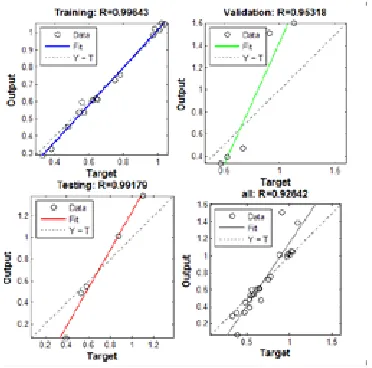
Fig. 8.
Performance of Network with R Value (R) (Original Inputs Vs Trip Rate (motorised))
Fig. 8 shows how the training, testing,
validation for data of original inputs against target data Trip Rate (motorised). Mean square error is 0.132 in 2 epochs.
Fig. 9.
Fig. 9 shows how the training, testing, validation for data of original inputs against target data Trip Rate (motorised). Mean square error is 0.010 in 3 epochs.
Comparative results of original and Principal Component Inputs Vs Trip Rate (motorised) are tabulated in Table 6.
Table 6
Comparative Results for Trip Rate (Motorised) as Target Data
Inputs Vs
motorised R MSE Epochs
PCA-6 0.96344 0.010 3
PCA-5 0.94494 0.003 2
PCA-4 0.93828 0.001 13
PCA-3 0.93698 0.017 5
Original
input 0.92642 0.132 2
R values for Inputs Vs Trip Rate (motorised) while using 6 PCA, 5 PCA, 4 PCA, 3 PCA are 0.963, 0.944, 0.938, 0.936 proving that PCA has a distinctive advantage over original inputs processed in ANN.
5. Conclusions
1. Using Principal Components with ANN proved to be an effective procedure as reduced inputs are more convenient for computation purpose without loss of information.
2. Using the selected data, Principal Component 1 is highly correlated with the parameters Population, City Area, Trip Length, Public Transport Share, City Buses, residential, industrial, recreational and transport area share. 3. The ANN model formed using the
original input data and trip-rate (all modes) suggested that there is a 90% agreement between the observed output and the modelled output.
4. The analysis of Trip Rate (all-modes) using 6 principal components as the inputs, resulted in the best correlation between the observed output and the
modelled output, when compared to the model formed with 5, 4 and 3 components. The R values are 0.964, 0.950, 0.941, 0.935 for 6 PCA, 5 PCA, 4 PCA, 3 PCA respectively.
5. The ANN model formed using the original input data and trip-rate (motorised) suggested that there is a 92% agreement between the observed output and the modelled output. 6. The analysis of Trip Rate (motorised)
using 6 principal components as the inputs, resulted in the best correlation between the observed output and the modelled output, when compared to the model formed with 5, 4 and 3 components. The R values are 0.963, 0.944, 0.938, 0.936 for 6 PCA, 5 PCA, 4 PCA, 3 PCA respectively, proving that PCA has a distinctive advantage over original inputs processed in ANN.
References
Burns, J.A.; Whitesides, G.M. 1993. Feed-forward neural networks in chemistry: mathematical systems for classification and pattern recognition, Chemical
Reviews 93(8): 2583-2601.
Gevrey, M.; Dimopoulos, I.; Lek, S. 2003. Review and comparison of methods to study the contribution of variables in artificial neural network models, Ecological
modeling 160(3): 249-264.
Kadali, B.R.; Rathi, N.; Perumal, V. 2014. Evaluation of pedestrian mid-block road crossing behaviour using artificial neural network, Journal of traffic and transportation engineering (English edition) 1(2): 111-119. Lyons, G.; Hunt, J.; McLeod, F. 2001. A neural network model for enhanced operation of midblock signalled pedestrian crossings, European journal of operational research 129(2): 346-354.
Manage, A.B.; Scariano, S.M. 2013. An introductory application of principal components to cricket data,
Journal of Statistics Education 21(3): 1-22.
Pau l, L .C.; Su ma n, A . A .; Su lta n, N. 2 013. Methodological analysis of principal component analysis (PCA) method, International Journal of Computational Engineering & Management 16(2): 32-38.
Pham, D.T.; Sagiroglu, S. 2001. Training multilayered perceptrons for pattern recognition: a comparative study of four training algorithms, International Journal
of Machine Tools and Manufacture 41(3): 419-430.